Batch OMP
In this section, we develop an efficient version of OMP known as Batch OMP [RZE08].
In OMP, given a signal \(\bar{y}\) and a dictionary \(\Phi\), our goal is to iteratively construct a sparse representation \(x\) such that \(\bar{y} \approx \Phi x\) satisfying either a target sparsity \(K\) of \(x\) or a target error \(\| \bar{y} - \Phi x\|_2 \leq \epsilon\). The algorithm picks an atom from \(\Phi\) in each iteration and computes a least squares estimate \(y\) of \(\bar{y}\) on the selected atoms. The residual \(r = \bar{y} - y\) is used to select the next atom by choosing the atom which matches best with the residual. Let \(I\) be the set of atoms selected in OMP after some iterations.
Recalling the OMP steps in the next iteration:
- Matching atoms with residuals: \(h = \Phi^T r\)
- Finding the new atom (best match with residual): \(i = \underset{j}{\text{arg max}} (\abs(h_j))\)
- Support update: \(I = I \cup \{ i \}\)
- Least squares: \(x_I = \Phi_I^{\dag} \bar{y}\)
- Approximation update: \(y = \Phi_I x_I = \Phi_I \Phi_I^{\dag} \bar{y}\)
- Residual update: \(r = \bar{y} - y = (I - \Phi_I \Phi_I^{\dag}) \bar{y}\)
Batch OMP is useful when we are trying to reconstruct representations of multiple signals at the same time.
Least Squares in OMP using Cholesky Update
Here we review how least squares can be fast implemented using Cholesky updates.
In the following, we will denote
- the matrix \(\Phi^T \Phi\) by the symbol \(G\)
- the matrix \(\Phi^T \Phi_I\) by the symbol \(G_I\)
- the matrix \((\Phi_I^T \Phi_I)\) by the symbol \(G_{I, I}\).
Note that \(G_I\) is formed by taking the columns indexed by \(I\) from \(G\). The matrix \(G_{I, I}\) is formed by taking the rows and columns both indexed by \(I\) from \(G\).
We have
and
We can rewrite:
If we perform a Cholesky decomposition of the Gram matrix \(G_{I, I} = \Phi_I^T \Phi_I\) as \(G_{I, I} = L L^T\), then we have:
Solving this equation involves
- Computing \(b = \Phi_I^T \bar{y}\)
- Solving the triangular system \(L u = b\)
- Solving the triangular system \(L^T x_I = u\)
We also need an efficient way of computing \(L\). It so happens that the Cholesky decomposition \(G_{I, I} = L L^T\) can be updated incrementally in each iteration of OMP. Let
- \(I^k\) denote the index set of chosen atoms after k iterations.
- \(\Phi_{I^k}\) denote the corresponding subdictionary of chosen atoms.
- \(G_{I^k, I^k}\) denote the Gram matrix \(\Phi_{I^k}^T \Phi_{I^k}\).
- \(L^k\) denote the Cholesky decomposition of G_{I^k, I^k}.
- \(i^k\) be the index of atom chosen in k-th iteration.
The Cholesky update process aims to compute \(L^k\) given \(L^{k-1}\) and \(i^k\). Note that we can write
Define \(v = \Phi_{I^{k-1}}^T \phi_{i^k}\). Note that \(\phi_{i^k}^T \phi_{i^k} = 1\) for dictionaries with unit norm columns. This gives us:
This can be solved to give us an equation for update of Cholesky decomposition:
where \(w\) is the solution of the triangular system \(L^{k - 1} w = v\).
Removing residuals from the computation
An interesting observation on OMP is that the real goal of OMP is to identify the index set of atoms participating in the sparse representation of \(\bar{y}\). The computation of residuals is just a way of achieving the same. If the index set has been identified, then the sparse representation is given by \(x_I = \Phi_I^{\dag} \bar{y}\) with all other entries in \(x\) set to zero and the sparse approximation of \(y\) is given by \(\Phi_I x_I\).
The selection of atoms doesn’t really need the residual explicitly. All it needs is a way to update the inner products of atoms in \(\Phi\) with the current residual. In this section, we will rewrite the OMP steps in a way that doesn’t require explicit computation of residual.
We begin with pre-computation of \(\bar{h} = \Phi^T \bar{y}\). This is the initial value of \(h\) (the inner products of atoms in dictionary with the current residual). This computation is anyway needed for OMP. Now, let’s expand the calculation of \(h\):
But \(\Phi_I^T \bar{y}\) is nothing but \(\bar{h}_I\). Thus,
This means that if \(\bar{h} = \Phi^T \bar{y}\) and \(G = \Phi^T \Phi\) have been precomputed, then \(h\) can be computed for each iteration without explicitly computing the residual.
If we are reconstructing just one signal, then the computation of \(G\) is very expensive. But, if we are reconstructing thousands of signals together in batch, computation of \(G\) is actually a minuscule factor in overall computation. This is the essential trick in Batch OMP algorithm.
There is one more issue to address. A typical halting criterion in OMP is the error based stopping criterion which compares the norm of the residual with a threshold. If the residual norm goes below the threshold, we stop OMP. If the residual is not computed explicitly, the it becomes challenging to apply this criterion. However, there is a way out. In the following, let
- \(x_{I^k} = \Phi_{I^k}^{\dag} \bar{y}\) be the non-zero entries in the k-th sparse representation
- \(x^k\) denote the k-th sparse representation
- \(y^k\) be the k-th sparse approximation \(y^k = \Phi x^k = \Phi_{I^k} x_{I^k}\)
- \(r^k\) be the residual \(\bar{y} - y^k\).
We start by writing a residual update equation. We have:
Combining the two, we get:
Due to the orthogonality of the residual, we have \(\langle r^k, y^k \rangle = 0\). Using this property and a long derivation (in eq 2.8 of [RZE08]), we obtain the relationship:
We introduce the symbols \(\epsilon^k = \| r^k \|_2^2\) and \(\delta^k = (x^k)^T G x^k\). The previous equation reduces to:
Thus, we just need to keep track of the quantity \(\delta^k\). Note that \(\delta^0 = 0\) since the initial estimate \(x^0 = 0\) for OMP.
Recall that
which has already been computed for updating \(h\) and can be reused. So
which is a simple inner product.
The Batch OMP Algorithm
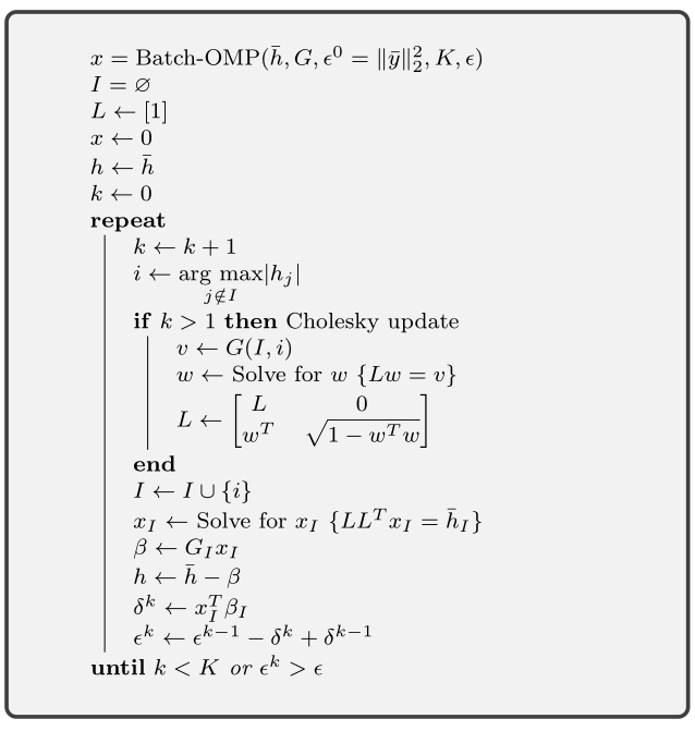
The batch OMP algorithm is described in the figure below.
The inputs are
- The Gram matrix \(G = \Phi^T \Phi\).
- The initial correlation vector \(\bar{h} = \Phi^T \bar{y}\).
- The squared norm \(\epsilon^0\) of the signal \(\bar{y}\) whose sparse representation we are constructing.
- The upper bound on the desired sparsity level \(K\)
- Residual norm (squared) threshold \(\epsilon\).
It returns the sparse representation \(x\).
Note that the algorithm doesn’t need direct access to either the dictionary \(\Phi\) or the signal \(\bar{y}\).
Note
The sparse vector \(x\) is usually returned as a pair of vectors \(I\) and \(x_I\). This is more efficient in terms of space utilization.
Fast Batch OMP Implementation
As part of sparse-plex, we provide a fast CPU based implementation of Batch OMP. It is up to 3 times faster than the Batch OMP implementation in OMPBOX.
This is written in C and uses the BLAS and LAPACK features available in MATLAB. The implementation is available in the function spx.fast.batch_omp. The corresponding C code is in batch_omp.c.
A Simple Example
Let’s create a Gaussian matrix (with normalized columns):
M = 400;
N = 1000;
Phi = spx.dict.simple.gaussian_mtx(M, N);
See Hands on with Gaussian sensing matrices for details.
Let’s create a few thousand sparse signals:
K = 16;
S = 5000;
X = spx.data.synthetic.SparseSignalGenerator(N, K, S).biGaussian();
See Generation of synthetic sparse representations for details.
Let’s compute their measurements using the Gaussian matrix:
Y = Phi*X;
We wish to recover \(X\) from \(Y\) and \(\Phi\).
Let’s precompute the Gram matrix:
G = Phi' * Phi;
Let’s precompute the correlation vectors for each signal:
DtY = Phi' * Y;
Let’s perform sparse recovery using Batch OMP and time it:
start_time = tic;
result = spx.fast.batch_omp(Phi, [], G, DtY, K, 1e-12);
elapsed_time = toc(start_time);
fprintf('Time taken: %.2f seconds\n', elapsed_time);
fprintf('Per signal time: %.2f usec', elapsed_time * 1e6/ S);

Time taken: 0.52 seconds
Per signal time: 103.18 usec
We note that the reconstruction has happened very quickly taking about just 100 micro seconds per signal.
We can verify the correctness of the result:
cmpare = spx.commons.SparseSignalsComparison(X, result, K);
cmpare.summarize();

Signal dimension: 1000
Number of signals: 5000
Combined reference norm: 536.04604784
Combined estimate norm: 536.04604784
Combined difference norm: 0.00000000
Combined SNR: 302.5784 dB

All signals have indeed been recovered correctly.
See :ref:`sec:library-commons-comparison-sparse` for
details about ``SparseSignalsComparison``.
For comparison, let’s see the time taken by Fast OMP implementation:
fprintf('Reconstruction with Fast OMP')
start_time = tic;
result = spx.fast.omp(Phi, Y, K, 1e-12);
elapsed_time = toc(start_time);
fprintf('Time taken: %.2f seconds\n', elapsed_time);
fprintf('Per signal time: %.2f usec', elapsed_time * 1e6/ S);

Reconstruction with Fast OMPTime taken: 4.39 seconds
Per signal time: 878.88 usec
See Fast Implementation of OMP for details about our fast OMP implementation.
Fast Batch OMP implementation is more than 8 times faster than fast OMP implementation for this problem configuration (M, N, K, S).
Benchmarks
| OS | Windows 7 Professional 64 Bit |
| Processor | Intel(R) Core(TM) i7-3630QM CPU @ 2.40GHz |
| Memory (RAM) | 16.0 GB |
| Hard Disk | SATA 120GB |
| MATLAB | R2017b |
The method for benchmarking has been adopted from
the file ompspeedtest.m in the OMPBOX
package by Ron Rubinstein.
We compare following algorithms:
- Batch OMP in OMPBOX.
- Our C version in sparse-plex.
The work load consists of a Gaussian dictionary of size \(512 \times 1000\). Sufficient signals are chosen so that the benchmarks can run reasonable duration. 8 sparse representations are constructed for each randomly generated signal in the given dictionary.
Speed summary for 178527 signals, dictionary size 512 x 1000:
Call syntax        Algorithm               Total time
--------------------------------------------------------
OMP(D,X,G,T)                     Batch-OMP               60.83 seconds
OMP(DtX,G,T)                     Batch-OMP with DTX    12.73 seconds
SPX-Batch-OMP(D, X, G, [], T)    SPX-Batch-OMP           19.78 seconds
SPX-Batch-OMP([], [], G, Dtx, T) SPX-Batch-OMP DTX      7.25 seconds
Gain SPX/OMPBOX without DTX 3.08
Gain SPX/OMPBOX with DTX 1.76
Our implementation is up to 3 times faster on this large workload.
The benchmark generation code is in ex_fast_batch_omp_speed_test.m.