Gaussian sensing matrices

In this section we collect several results related to Gaussian sensing matrices.

Definition

A Gaussian sensing matrix \(\Phi \in \RR^{M \times N}\) with \(M < N\) is constructed by drawing each entry \(\phi_{ij}\) independently from a Gaussian random distribution \(\Gaussian(0, \frac{1}{M})\) .

We note that

\[\EE(\phi_{ij}) = 0.\]

\[\EE(\phi_{ij}^2) = \frac{1}{M}.\]

We can write

\[\Phi = \begin{bmatrix} \phi_1 & \dots & \phi_N \end{bmatrix}\]

where \(\phi_j \in \RR^M\) is a Gaussian random vector with independent entries.

We note that

\[\EE (\| \phi_j \|_2^2) = \EE \left ( \sum_{i=1}^M \phi_{ij}^2 \right ) = \sum_{i=1}^M (\EE (\phi_{ij}^2)) = M \frac{1}{M} = 1.\]

Thus the expected value of squared length of each of the columns in \(\Phi\) is \(1\) .

Joint correlation

Columns of \(\Phi\) satisfy a joint correlation property ([TG07]) which is described in following lemma.

Lemma

Let \(\{u_k\}\) be a sequence of \(K\) vectors (where \(u_k \in \RR^M\) ) whose \(l_2\) norms do not exceed one. Independently choose \(z \in \RR^M\) to be a random vector with i.i.d. \(\Gaussian(0, \frac{1}{M})\) entries. Then

\[\PP\left(\max_{k} | \langle z, u_k\rangle | \leq \epsilon \right) \geq 1 - K \exp \left( - \epsilon^2 \frac{M}{2} \right).\]

Proof

Let us call \(\gamma = \max_{k} | \langle z, u_k\rangle |\) .

We note that if for any \(u_k\) , \(\| u_k \|_2 <1\) and we increase the length of \(u_k\) by scaling it, then \(\gamma\) will not decrease and hence \(\PP(\gamma \leq \epsilon)\) will not increase. Thus if we prove the bound for vectors \(u_k\) with \(\| u_k\|_2 = 1 \Forall 1 \leq k \leq K\) , it will be applicable for all \(u_k\) whose \(l_2\) norms do not exceed one. Hence we will assume that \(\| u_k \|_2 = 1\) .

Now consider \(\langle z, u_k \rangle\) . Since \(z\) is a Gaussian random vector, hence \(\langle z, u_k \rangle\) is a Gaussian random variable. Since \(\| u_k \| =1\) hence

\[\langle z, u_k \rangle \sim \Gaussian \left(0, \frac{1}{M} \right).\]

We recall a well known tail bound for Gaussian random variables which states that

\[\PP_X ( | x | > \epsilon) \; = \; \sqrt{\frac{2}{\pi}} \int_{\epsilon \sqrt{N}}^{\infty} \exp \left( -\frac{x^2}{2}\right) d x \; \leq \; \exp \left (- \epsilon^2 \frac{M}{2} \right).\]

Now the event

\[\left \{ \max_{k} | \langle z, u_k\rangle | > \epsilon \right \} = \bigcup_{ k= 1}^K \{| \langle z, u_k\rangle | > \epsilon\}\]

i.e. if any of the inner products (absolute value) is greater than \(\epsilon\) then the maximum is greater.

We recall Boole’s inequality which states that

\[\PP \left(\bigcup_{i} A_i \right) \leq \sum_{i} \PP(A_i).\]

Thus

\[\PP\left(\max_{k} | \langle z, u_k\rangle | > \epsilon \right) \leq K \exp \left(- \epsilon^2 \frac{M}{2} \right).\]

This gives us

\[\begin{split}\begin{aligned} \PP\left(\max_{k} | \langle z, u_k\rangle | \leq \epsilon \right) &= 1 - \PP\left(\max_{k} | \langle z, u_k\rangle | > \epsilon \right) \\ &\geq 1 - K \exp \left(- \epsilon^2 \frac{M}{2} \right). \end{aligned}\end{split}\]

Hands on with Gaussian sensing matrices

We will show several examples of working with Gaussian sensing matrices through the sparse-plex library.

ExampleConstructing a Gaussian sensing matrix

Let’s specify the size of representation space:

N = 1000;

Let’s specify the number of measurements:

M = 100;

Let’s construct the sensing matrix:

Phi = spx.dict.simple.gaussian_mtx(M, N, false);

By default the function gaussian_mtx constructs a matrix with normalized columns. When we set the third argument to false as in above, it constructs a matrix with unnormalized columns.

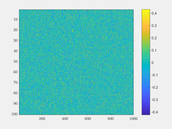
We can visualize the matrix easily:

imagesc(Phi);
colorbar;

Let’s compute the norms of each of the columns:

column_norms = spx.norm.norms_l2_cw(Phi);

Let’s look at the mean value:

>> mean(column_norms)

ans =

    0.9942

We can see that the mean value is very close to unity as expected.

Let’s compute the standard deviation:

>> std(column_norms)

ans =

    0.0726

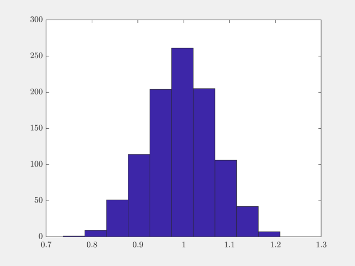
As expected, the column norms are concentrated around its mean.

We can examine the variation in norm values by looking at the quantile values:

>> quantile(column_norms, [0.1, 0.25, 0.5, 0.75, 0.9])

ans =

    0.8995    0.9477    0.9952    1.0427    1.0871

The histogram of column norms can help us visualize it better:

hist(column_norms);

The singular values of the matrix help us get deeper understanding of how well behaved the matrix is:

singular_values = svd(Phi);
figure;
plot(singular_values);
ylim([0, 5]);
grid;

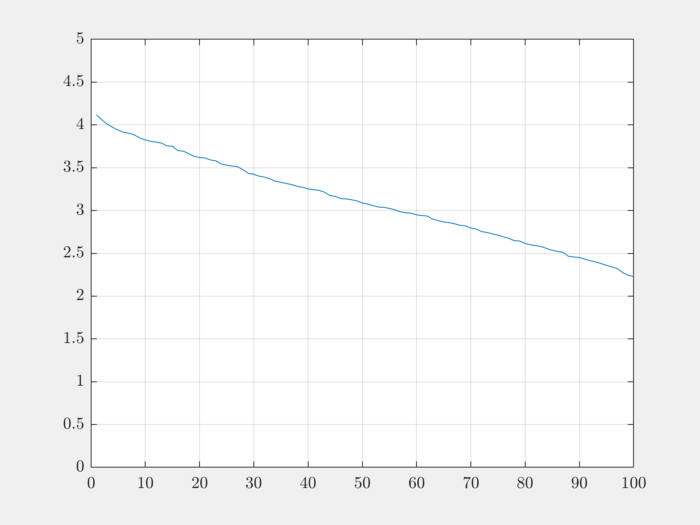
As we can see, singular values decrease quite slowly.

The condition number captures the variation in singular values:

>> max(singular_values)

ans =

    4.1177

>> min(singular_values)

ans =

    2.2293

>> cond(Phi)

ans =

    1.8471

The source code can be downloaded here.