The OMP Algorithm¶

Orthogonal Matching Pursuit (OMP) addresses some of the limitations of Matching Pursuit. In particular, in each iteration:

The current estimate is computed by performing a least squares estimation on the subdictionary formed by atoms selected so far.
It ensures that the residual is totally orthogonal to already selected atoms.
It also means that an atom is selected only once.
Further, if all the atoms in the support are selected by OMP correctly, then the least squares estimate is able to achieve perfect recovery. The residual becomes 0.
In other words, if OMP is recovering a K-sparse representation, then it can recover it in exactly K iterations (if in each iteration it recovers one atom correctly).
OMP performs far better than MP in terms of the set of signals it can recover correctly.
At the same time, OMP is a much more complex algorithm (due to the least squares step).

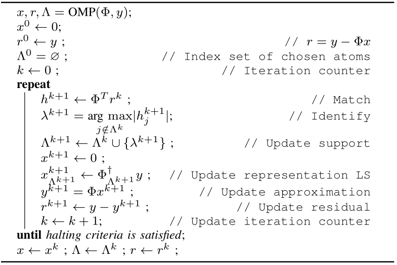
Orthogonal Matching Pursuit

The core OMP algorithm is presented above. The algorithm is iterative.

We start with the initial estimate of solution as \(x=0\).
We also maintain the support of \(x\) i.e. the set of indices for which \(x\) is non-zero in a variable \(\Lambda\). We start with an empty support.
In each (\(k\)-th) iteration we attempt to reduce the difference between the actual signal \(y\) and the approximate signal based on current solution \(x^{k}\) given by \(r^{k} = y - \Phi x^{k}\).
We do this by choosing a new index in \(x\) given by \(\lambda^{k+1}\) for the column \(\phi_{\lambda^{k+1}}\) which most closely matches our current residual.
We include this to our support for \(x\), estimate new solution vector \(x^{k+1}\) and compute new residual.
We stop when the residual magnitude is below a threshold \(\epsilon\) defined by us.

Each iteration of algorithm consists of following stages:

Match For each column \(\phi_j\) in our dictionary, we measure the projection of residual from previous iteration on the column
Identify We identify the atom with largest inner product and store its index in the variable \(\lambda^{k+1}\).
Update support We include \(\lambda^{k+1}\) in the support set \(\Lambda^{k}\).
Update representation In this step we find the solution of minimizing \(\| \Phi x - y \|^2\) over the support \(\Lambda^{k+1}\) as our next candidate solution vector.

By keeping \(x_i = 0\) for \(i \notin \Lambda^{k+1}\) we are essentially leaving out corresponding columns \(\phi_i\) from our calculations.

Thus we pickup up only the columns specified by \(\Lambda^{k+1}\) from \(\Phi\). Let us call this matrix as \(\Phi_{\Lambda^{k+1}}\). The size of this matrix is \(N \times | \Lambda^{k+1} |\). Let us call corresponding sub vector as \(x_{\Lambda^{k+1}}\).

E.g. suppose \(D=4\), then \(\Phi = \begin{bmatrix} \phi_1 & \phi_2 & \phi_3 & \phi_4 \end{bmatrix}\). Let \(\Lambda^{k+1} = \{1, 4\}\). Then \(\Phi_{\Lambda^{k+1}} = \begin{bmatrix} \phi_1 & \phi_4 \end{bmatrix}\) and \(x_{\Lambda^{k+1}} = (x_1, x_4)\).

Our minimization problem then reduces to minimizing \(\|\Phi_{\Lambda^{k+1}} x_{\Lambda^{k+1}} - y \|_2\).

We use standard least squares estimate for getting the coefficients for \(x_{\Lambda^{k+1}}\) over these indices. We put back \(x_{\Lambda^{k+1}}\) to obtain our new solution estimate \(x^{k+1}\).

In the running example after obtaining the values \(x_1\) and \(x_4\), we will have \(x^{k+1} = (x_1, 0 , 0, x_4)\).

The solution to this minimization problem is given by

\[\Phi_{\Lambda^{k+1}}^H ( \Phi_{\Lambda^{k+1}}x_{\Lambda^{k+1}} - y ) = 0 \implies x_{\Lambda^{k+1}} = ( \Phi_{\Lambda^{k+1}}^H \Phi_{\Lambda^{k+1}} )^{-1} \Phi_ {\Lambda^{k+1}}^H y.\]

Interestingly, we note that \(r^{k+1} = y - \Phi x^{k+1} = y - \Phi_{\Lambda^{k+1}} x_{\Lambda^{k+1}}\), thus

\[\Phi_{\Lambda^{k+1}}^H r^{k+1} = 0\]

which means that columns in \(\Phi_{\Lambda^k}\) which are part of support \(\Lambda^{k+1}\) are necessarily orthogonal to the residual \(r^{k+1}\). This implies that these columns will not be considered in the coming iterations for extending the support. This orthogonality is the reason behind the name of the algorithm as OMP.
Update residual We finally update the residual vector to \(r^{k+1}\) based on new solution vector estimate.

Hands-on with Orthogonal Matching Pursuit¶

Example

Let us consider a synthesis matrix of size \(10 \times 20\). Thus \(N=10\) and \(D=20\). In order to fit into the display, we will present the matrix in two 10 column parts.

tiny

\[\begin{split}\begin{aligned} \Phi_a = \frac{1}{\sqrt{10}} \begin{bmatrix} -1 & -1 & -1 & 1 & -1 & -1 & 1 & 1 & -1 & 1\\ 1 & 1 & 1 & 1 & 1 & -1 & -1 & 1 & -1 & -1\\ -1 & -1 & -1 & -1 & -1 & 1 & 1 & 1 & 1 & 1\\ 1 & -1 & -1 & 1 & 1 & 1 & -1 & 1 & 1 & 1\\ 1 & 1 & 1 & -1 & -1 & 1 & -1 & -1 & 1 & 1\\ 1 & -1 & 1 & -1 & -1 & -1 & 1 & -1 & 1 & -1\\ -1 & -1 & 1 & 1 & -1 & -1 & -1 & -1 & 1 & -1\\ 1 & -1 & 1 & 1 & -1 & 1 & -1 & -1 & -1 & 1\\ -1 & 1 & -1 & 1 & 1 & -1 & -1 & -1 & 1 & 1\\ 1 & 1 & 1 & 1 & -1 & 1 & -1 & 1 & -1 & 1 \end{bmatrix}\\ \Phi_b = \frac{1}{\sqrt{10}} \begin{bmatrix} 1 & -1 & -1 & -1 & 1 & 1 & 1 & -1 & -1 & -1\\ 1 & 1 & 1 & -1 & -1 & -1 & -1 & -1 & -1 & 1\\ -1 & 1 & 1 & 1 & 1 & 1 & -1 & -1 & -1 & -1\\ 1 & -1 & 1 & -1 & 1 & 1 & 1 & -1 & -1 & -1\\ 1 & -1 & -1 & 1 & 1 & 1 & -1 & 1 & 1 & -1\\ -1 & 1 & 1 & 1 & -1 & 1 & -1 & 1 & -1 & 1\\ -1 & 1 & 1 & -1 & 1 & -1 & -1 & -1 & 1 & 1\\ 1 & -1 & -1 & 1 & 1 & -1 & -1 & 1 & -1 & 1\\ 1 & 1 & 1 & 1 & -1 & -1 & 1 & 1 & 1 & -1\\ -1 & -1 & 1 & 1 & -1 & 1 & 1 & -1 & -1 & 1 \end{bmatrix} \end{aligned}\end{split}\]

with

\[\Phi = \begin{bmatrix}\Phi_a & \Phi_b \end{bmatrix}.\]

You may verify that each column is unit norm.

It is known that \(\Rank(\Phi) = 10\) and \(\spark(\Phi)= 6\). Thus if a signal \(y\) has a \(2\) sparse representation in \(\Phi\) then the representation is necessarily unique.

We now consider a signal \(y\) given by

\[\begin{split}\small y = \begin{pmatrix} 4.74342 & -4.74342 & 1.58114 & -4.74342 & -1.58114 \\ 1.58114 & -4.74342 & -1.58114 & -4.74342 & -4.74342 \end{pmatrix}. \normalsize\end{split}\]

For saving space, we have written it as an n-tuple over two rows. You should treat it as a column vector of size \(10 \times 1\).

It is known that the vector has a two sparse representation in \(\Phi\). Let us go through the steps of OMP and see how it works.

In step 0, \(r^0= y\), \(x^0 = 0\), and \(\Lambda^0 = \EmptySet\).

We now compute absolute value of inner product of \(r^0\) with each of the columns. They are given by

\[\begin{split}\small \begin{pmatrix} 4 & 4 & 4 & 7 & 3 & 1 & 11 & 1 & 2 & 1 \\ 2 & 1 & 7 & 0 & 2 & 4 & 0 & 2 & 1 & 3 \end{pmatrix} \normalsize\end{split}\]

We quickly note that the maximum occurs at index 7 with value 11.

We modify our support to \(\Lambda^1 = \{ 7 \}\).

We now solve the least squares problem

\[\text{minimize} \left \| y - [\phi_7] x_7 \right \|_2^2.\]

The solution gives us \(x_7 = 11.00\). Thus we get

\[\begin{split}x^1 = \begin{pmatrix} 0 & 0 & 0 & 0 & 0 & 0 & 11 & 0 & 0 & 0 \\ 0 & 0 & 0 & 0 & 0 & 0 & 0 & 0 & 0 & 0 \end{pmatrix}.\end{split}\]

Again note that to save space we have presented \(x\) over two rows. You should consider it as a \(20 \times 1\) column vector.

This leaves us the residual as

\[\begin{split}r^1 = y - \Phi x^1 = \begin{pmatrix} 1.26491 & -1.26491 & -1.89737 & -1.26491 & 1.89737 \\ -1.89737 & -1.26491 & 1.89737 & -1.26491 & -1.26491 \end{pmatrix}.\end{split}\]

We can cross check that the residual is indeed orthogonal to the columns already selected, for

\[\langle r^1 , \phi_7 \rangle = 0.\]

Next we compute inner product of \(r^1\) with all the columns in \(\Phi\) and take absolute values. They are given by

\[\begin{split}\begin{pmatrix} 0.4 & 0.4 & 0.4 & 0.4 & 0.8 & 1.2 & 0 & 1.2 & 2 & 1.2 \\ 2.4 & 3.2 & 4.8 & 0 & 2 & 0.4 & 0 & 2 & 1.2 & 0.8 \end{pmatrix}\end{split}\]

We quickly note that the maximum occurs at index 13 with value \(4.8\).

We modify our support to \(\Lambda^1 = \{ 7, 13 \}\).

We now solve the least squares problem

\[\begin{split}\text{minimize} \left \| y - \begin{bmatrix} \phi_7 & \phi_{13} \end{bmatrix} \begin{bmatrix} x_7 \\ x_{13} \end{bmatrix} \right \|_2^2.\end{split}\]

This gives us \(x_7 = 10\) and \(x_{13} = -5\).

Thus we get

\[\begin{split}x^2 = \begin{pmatrix} 0 & 0 & 0 & 0 & 0 & 0 & 10 & 0 & 0 & 0 \\ 0 & 0 & -5 & 0 & 0 & 0 & 0 & 0 & 0 & 0 \end{pmatrix}\end{split}\]

Finally the residual we get at step 2 is

\[\begin{split}r^2 = y - \Phi x^2 = 10^{-14} \begin{pmatrix} 0 & 0 & -0.111022 & 0 & 0.111022 \\ -0.111022 & 0 & 0.111022 & 0 & 0 \end{pmatrix}\end{split}\]

The magnitude of residual is very small. We conclude that our OMP algorithm has converged and we have been able to recover the exact 2 sparse representation of \(y\) in \(\Phi\).