Framework for study of performance of pursuit algorithms

Experimental study of pursuit algorithms for sparse recovery needs following components:

• Generation of synthetic sparse representations
• Generation of synthetic compressible representations
• Addition of measurement error
• Measurement of recovery error
• Phase transition diagrams

sparse-plex library provides a wide variety of functions to help with the study of pursuit algorithms.

Generation of synthetic sparse representations

A sparse representation is constructed in an appropriate representation space.

The class spx.data.synthetic.SparseSignalGenerator provides various methods for generating synthetic sparse representations from different distributions.

• Uniform
• Bi-uniform
• Gaussian
• Complex Gaussian
• Rademacher
• Bi-Gaussian
• Real spherical rows
• Complex spherical rows

It takes following parameters:

\(N\)

The dimension of the representation space

\(K\)

The sparsity level of representations

\(S\) (optional)

Number of sparse representations to generate with a common support. Default value is 1.

The generator first uniformly selects a random support of \(K\) indices from the index set \([1, N]\).

After that it provides various ways to generate the non-zero values.

Uniform

ExampleSparse representations with uniformly distributed non-zero values

We create the sparse signal generator instance:

N = 32;
K = 4;
gen = spx.data.synthetic.SparseSignalGenerator(N, K);

We generate a sparse vector:

rep =  gen.uniform();

Let’s plot it:

stem(rep, '.');

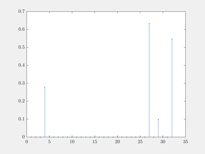
Note that all non-zero entries are positive and they are distributed uniformly between \([0, 1]\).

We can easily identify the support for the representation:

>> spx.commons.sparse.support(rep)'

ans =

     4    27    29    32

The \(\ell_0\)-“norm” can be calculated easily too:

>> spx.commons.sparse.l0norm(rep)

ans =

     4

Let’s cross-check with the support used by the generator:

>> gen.Omega

ans =

    27    29     4    32

By default, non-zero values are chosen between the range \([0, 1]\).

We can specify a custom range \([a, b]\) by calling:

rep =  gen.uniform(a, b);

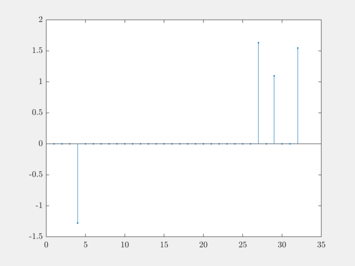
Bi-uniform

The problem with previous example is that all non-zero entries are positive. We would like that the sign of non-zero entries also changes with equal probability. This can be achieved using bi-uniform generator.

• The non-zero values are generated using uniform distribution.
• A sign for each non-zero entry is chosen with equal probability.
• The sign is multiplied to the non-zero value.

ExampleSparse representations with bi-uniformly distributed non-zero values

The setup steps are same:

N = 32;
K = 4;
gen = spx.data.synthetic.SparseSignalGenerator(N, K);

The representation generation step changes:

rep =  gen.biUniform();

Plotting:

stem(rep, '.');

ExampleChanging the range of values

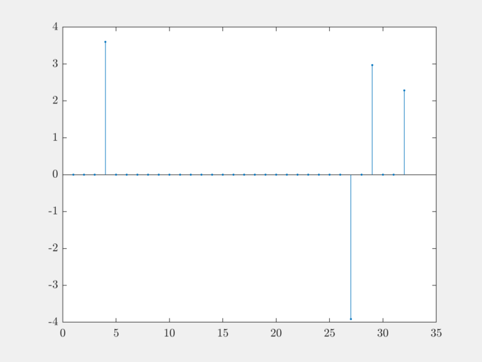
We will generate the magnitudes between 2 and 4:

rep =  gen.biUniform(2, 4);

Plotting:

stem(rep, '.');

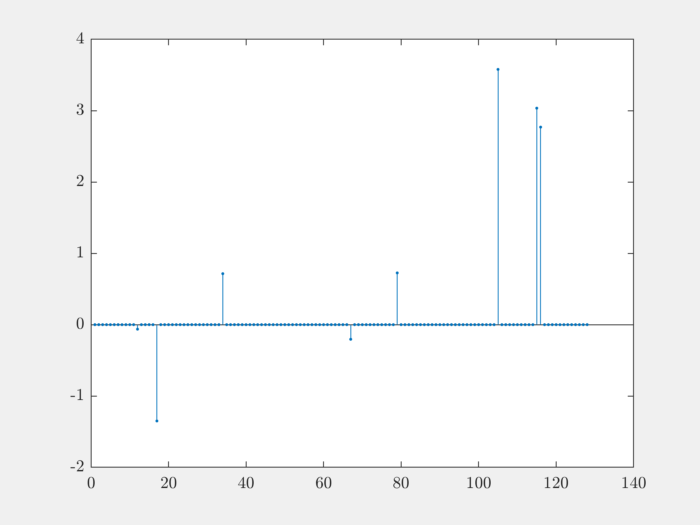
Gaussian

ExampleSparse representations with Gaussian distributed non-zero values

Let’s increase the dimensions of our representation space and sparsity level:

N = 128;
K = 8;
gen = spx.data.synthetic.SparseSignalGenerator(N, K);

Let’s generate non-zero entries using Gaussian distribution:

rep =  gen.gaussian();

Plot it:

stem(rep, '.');

Bi-Gaussian

While the non-zero values in Gaussian distribution have both signs, we can see that some of the non-zero values are way too small. These are problematic for those sparse recovery algorithms which are not very good with way too small values or which demand that the dynamic range between the large non-zero values and small non-zero values shouldn’t be too high. The small non-zero values are also problematic in the presence of noise as it is hard to distinguish them from noise.

To address these concerns, we have a bi-Gaussian distribution.

The way it works is as follows:

• Generate non-zero values using Gaussian distribution.
• Let a value be \(x\).
• Let an offset \(\alpha > 0\) be given.
• If \(x > 0\), then \(x = x + \alpha\).
• If \(x < 0\), then \(x = x - \alpha\).

Default value of offset is 1.

ExampleSparse representations with bi-Gaussian distributed non-zero values

Setup:

N = 128;
K = 8;
gen = spx.data.synthetic.SparseSignalGenerator(N, K);

Generating the representation vector:

rep =  gen.biGaussian();

Plot it:

stem(rep, '.');

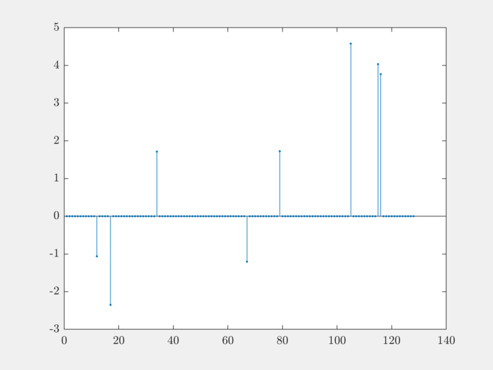
Let’s pickup the non-zero values from this vector:

>> nz_rep = rep(rep~=0)'; nz_rep

nz_rep =

   -1.0631   -2.3499    1.7147   -1.2050    1.7254    4.5784    4.0349    3.7694

Let’s estimate the dynamic range:

>> anz_rep = abs(nz_rep);
>> dr = max(anz_rep) / min(anz_rep)

dr =

    4.3068

The bi-Gaussian distribution is quite flexible.

• The non-zero values are both positive and negative.
• Quite large non-zero values are possible (though rare).
• Too small values are not allowed.
• Dynamic range between largest and smallest non-zero values is not much.

Rademacher

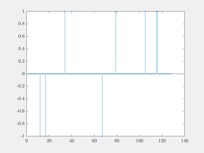
Sometimes, you want a sparse representation where the non-zero values are either \(+1\) or \(-1\). In this case, the non-zero values should be drawn from Rademacher distribution.

ExampleSparse representations with Rademacher distributed non-zero values

Setup:

N = 128;
K = 8;
gen = spx.data.synthetic.SparseSignalGenerator(N, K);

Generating Rademacher distributed non-zero values:

rep =  gen.rademacher();

Plot it:

stem(rep, '.');

Generating compressible signals

[Cev09] describes a set of probability distributions, dubbed compressible priors whose independent and identically distributed realizations result in p-compressible signals.

The authors provided a Matlab function randcs.m for generating compressible signals. It is included in sparse-plex.