Sparse solutions for under-determined linear systems

The discussion in this section is largely based on chapter 1 of [Ela10].

Consider a matrix \(\Phi \in \CC^{M \times N}\) with \(M < N\).

Define an under-determined system of linear equations:

\[\Phi x = y\]

where \(y \in \CC^M\) is known and \(x \in \CC^N\) is unknown.

This system has \(N\) unknowns and \(M\) linear equations. There are more unknowns than equations.

Let the columns of \(\Phi\) be given by \(\phi_1, \phi_2, \dots, \phi_N\).

Column space of \(\Phi\) (vector space spanned by all columns of \(\Phi\)) is denoted by \(\ColSpace(\Phi)\) i.e.

\[\ColSpace(\Phi) = \sum_{i=1}^{N} c_i \phi_i, \quad c_i \in \CC.\]

We know that \(\ColSpace(\Phi) \subset \CC^M\).

Clearly \(\Phi x \in \ColSpace(\Phi)\) for every \(x \in \CC^N\). Thus if \(y \notin \ColSpace(\Phi)\) then we have no solution. But, if \(y \in \ColSpace(\Phi)\) then we have infinite number of solutions.

Let \(\NullSpace(\Phi)\) represent the null space of \(\Phi\) given by

\[\NullSpace(\Phi) = \{ x \in \CC^N : \Phi x = 0\}.\]

Let \(\widehat{x}\) be a solution of \(y = \Phi x\). And let \(z \in \NullSpace(\Phi)\). Then

\[\Phi (\widehat{x} + z) = \Phi \widehat{x} + \Phi z = y + 0 = y.\]

Thus the set \(\widehat{x} + \NullSpace(\Phi)\) forms the complete set of infinite solutions to the problem \(y = \Phi x\) where

\[\widehat{x} + \NullSpace(\Phi) = \{\widehat{x} + z \quad \Forall z \in \NullSpace(\Phi)\}.\]

ExampleAn under-determined system

As a running example in this section, we will consider a simple under-determined system in \(\RR^2\). The system is specified by

\[\Phi = \begin{bmatrix} 3 & 4 \end{bmatrix}\]

and

\[\begin{split}x = \begin{bmatrix} x_1 \\ x_2 \end{bmatrix}\end{split}\]

with

\[\Phi x = y = 12.\]

where \(x\) is unknown and \(y\) is known. Alternatively

\[\begin{split}\begin{bmatrix} 3 & 4 \end{bmatrix} \begin{bmatrix} x_1 \\ x_2 \end{bmatrix} = 12\end{split}\]

or more simply

\[3 x_1 + 4 x_2 = 12.\]

The solution space of this system is a line in \(\RR^2\) which is shown in the figure below.

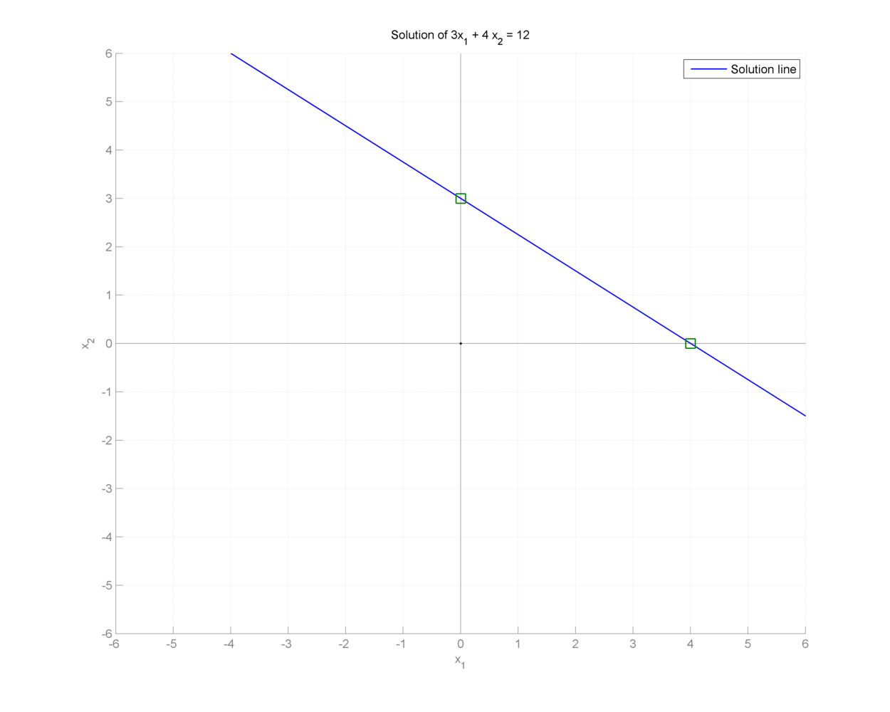
Specification of the under-determined system as above, doesn’t give us any reason to prefer one particular point on the line as the preferred solution.

Two specific solutions are of interest:

• \((x_1, x_2) = (4,0)\) lies on the \(x_1\) axis.
• \((x_1, x_2) = (0,3)\) lies on the \(x_2\) axis.

In both of these solutions, one component is 0, thus leading these solutions to be sparse.

It is easy to visualize sparsity in this simplified 2-dimensional setup but situation becomes more difficult when we are looking at high dimensional signal spaces. We need well defined criteria to promote sparse solutions.

Regularization

Are all these solutions equivalent or can we say that one solution is better than the other in some sense? In order to suggest that some solution is better than other solutions, we need to define a criteria for comparing two solutions.

In optimization theory, this idea is known as regularization.

We define a cost function \(J(x) : \CC^N \to \RR\) which defines the desirability of a given solution \(x\) out of infinitely possible solutions. The higher the cost, lower is the desirability of the solution.

Thus the goal of the optimization problem is to find a desired \(x\) with minimum possible cost.

In optimization literature, the cost function is one type of objective function. While the objective of an optimization problem might be either minimized or maximized, cost is always minimized.

We can write this optimization problem as

\[\begin{split}\begin{aligned} & \underset{x}{\text{minimize}} & & J(x) \\ & \text{subject to} & & y = \Phi x. \end{aligned}\end{split}\]

If \(J(x)\) is convex, then its possible to find a global minimum cost solution over the solution set.

If \(J(x)\) is not convex, then it may not be possible to find a global minimum, we may have to settle with a local minimum.

A variety of such cost function based criteria can be considered.

\(l_2\) Regularization

One of the most common criteria is to choose a solution with the smallest \(l_2\) norm.

The problem can then be reformulated as an optimization problem

\[\begin{split}\begin{aligned} & \underset{x}{\text{minimize}} & & \| x \|_2 \\ & \text{subject to} & & y = \Phi x. \end{aligned}\end{split}\]

In fact minimizing \(\| x \|_2\) is same as minimizing its square \(\| x \|_2^2 = x^H x\).

So an equivalent formulation is

\[\begin{split}\begin{aligned} & \underset{x}{\text{minimize}} & & x^H x \\ & \text{subject to} & & y = \Phi x. \end{aligned}\end{split}\]

ExampleMinimum :math:`l_2` norm solution for an under-determined system

We continue with our running example.

We can write \(x_2\) as

\[\]

x_2 = 3 - frac{3}{4} x_1.

With this definition the squared \(l_2\) norm of \(x\) becomes

\[\begin{split}\| x \|_2^2 = x_1^2 + x_2^2 &= x_1^2 + \left ( 3 - \frac{3}{4} x_1 \right )^2\\ & = \frac{25}{16} x_1^2 - \frac{9}{2} x_1 + 9.\end{split}\]

Minimizing \(\| x \|_2^2\) over all \(x\) is same as minimizing over all \(x_1\).

Since \(\| x \|_2^2\) is a quadratic function of \(x_1\), we can simply differentiate it and equate to 0 giving us

\[\frac{25}{8} x_1 - \frac{9}{2} = 0 \implies x_1 = \frac{36}{25} = 1.44.\]

This gives us

\[x_2 = \frac{48}{25} = 1.92.\]

Thus the optimal \(l_2\) norm solution is obtained at \((x_1, x_2) = (1.44, 1.92)\).

We note that the minimum \(l_2\) norm at this solution is

\[\| x \|_2 = \frac{12}{5} = 2.4.\]

It is instructive to note that the \(l_2\) norm cost function prefers a non-sparse solution to the optimization problem.

We can view this solution graphically by drawing \(l_2\) norm balls of different radii in figure below. The ball which just touches the solution space line (i.e. the line is tangent to the ball) gives us the optimal solution.

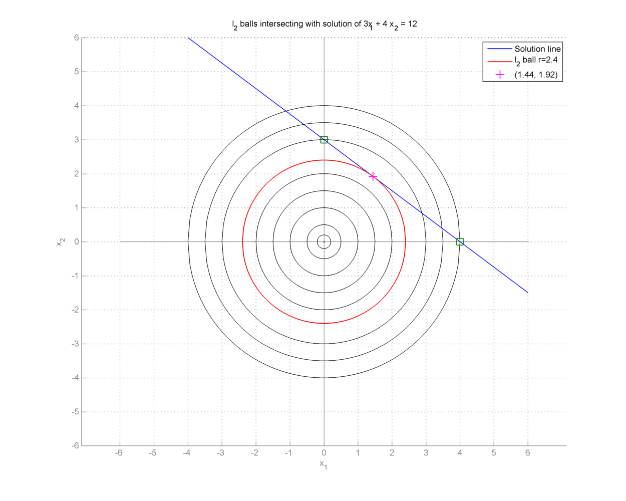
All other norm balls either don’t touch the solution line at all, or they cross it at exactly two points.

A formal solution to \(l_2\) norm minimization problem can be easily obtained using Lagrange multipliers.

We define the Lagrangian

\[\mathcal{L}(x) = \|x\|_2^2 + \lambda^H (\Phi x - y)\]

with \(\lambda \in \CC^M\) being the Lagrange multipliers for the (equality) constraint set.

Differentiating \(\mathcal{L}(x)\) w.r.t. \(x\) we get

\[\frac{\partial \mathcal{L}(x)} {\partial x} = 2 x + \Phi^H \lambda.\]

By equating the derivative to \(0\) we obtain the optimal value of \(x\) as

\[x^* = - \frac{1}{2} \Phi^H \lambda. \label{eq:ssm:underdetermined_l2_optimal_value_expression_1}\]

Plugging this solution back into the constraint \(\Phi x= y\) gives us

\[\Phi x^* = - \frac{1}{2} (\Phi \Phi^H) \lambda= y\implies \lambda = -2(\Phi \Phi^H)^{-1} y.\]

In above we are implicitly assuming that \(\Phi\) is a full rank matrix thus, \(\Phi \Phi^H\) is invertible and positive definite.

Putting \(\lambda\) back in above we obtain the well known closed form least squares solution using pseudo-inverse solution

\[x^* = \Phi^H (\Phi \Phi^H)^{-1} y = \Phi^{\dag} y.\]

We would like to mention that there are several iterative approaches to solve the \(l_2\) norm minimization problem (like gradient descent and conjugate descent). For large systems, they are more effective than computing the pseudo-inverse.

The beauty of \(l_2\) norm minimization lies in its simplicity and availability of closed form analytical solutions. This has led to its prevalence in various fields of science and engineering. But \(l_2\) norm is by no means the only suitable cost function. Rather the simplicity of \(l_2\) norm often drives engineers away from trying other possible cost functions. In the sequel, we will look at various other possible cost functions.

Convexity

Convex optimization problems have a unique feature that it is possible to find the global optimal solution if such a solution exists.

The solution space \(\Omega = \{x : \Phi x = y\}\) is convex. Thus the feasible set of solutions for the optimization problem is also convex. All it remains is to make sure that we choose a cost function \(J(x)\) which happens to be convex. This will ensure that a global minimum can be found through convex optimization techniques. Moreover, if \(J(x)\) is strictly convex, then it is guaranteed that the global minimum solution is unique. Thus even though, we may not have a nice looking closed form expression for the solution of a strictly convex cost function minimization problem, the guarantee of the existence and uniqueness of solution as well as well developed algorithms for solving the problem make it very appealing to choose cost functions which are convex.

We remind that all \(l_p\) norms with \(p \geq 1\) are convex functions. In particular \(l_{\infty}\) and \(l_1\) norms are very interesting and popular where

\[l_{\infty}(x) = \max(x_i), \, 1 \leq i \leq N\]

and

\[l_1(x) = \sum_{i=1}^{N} |x_i|.\]

In the following section we will attempt to find a unique solution to our optimization problem using \(l_1\) norm.

\(l_1\) Regularization

In this section we will restrict our attention to the Euclidean space case where \(x \in \RR^N\), \(\Phi \in \RR^{M \times N}\) and \(y \in \RR^M\).

We choose our cost function \(J(x) = l_1(x)\).

The cost minimization problem can be reformulated as

\[\begin{split}\begin{aligned} & \underset{x}{\text{minimize}} & & \| x \|_1 \\ & \text{subject to} & & \Phi x = y. \end{aligned}\end{split}\]

ExampleMinimum :math:`l_1` norm solution for an under-determined system

We continue with our running example.

Again we can view this solution graphically by drawing \(l_1\) norm balls of different radii in the figure below. The ball which just touches the solution space line gives us the optimal solution.

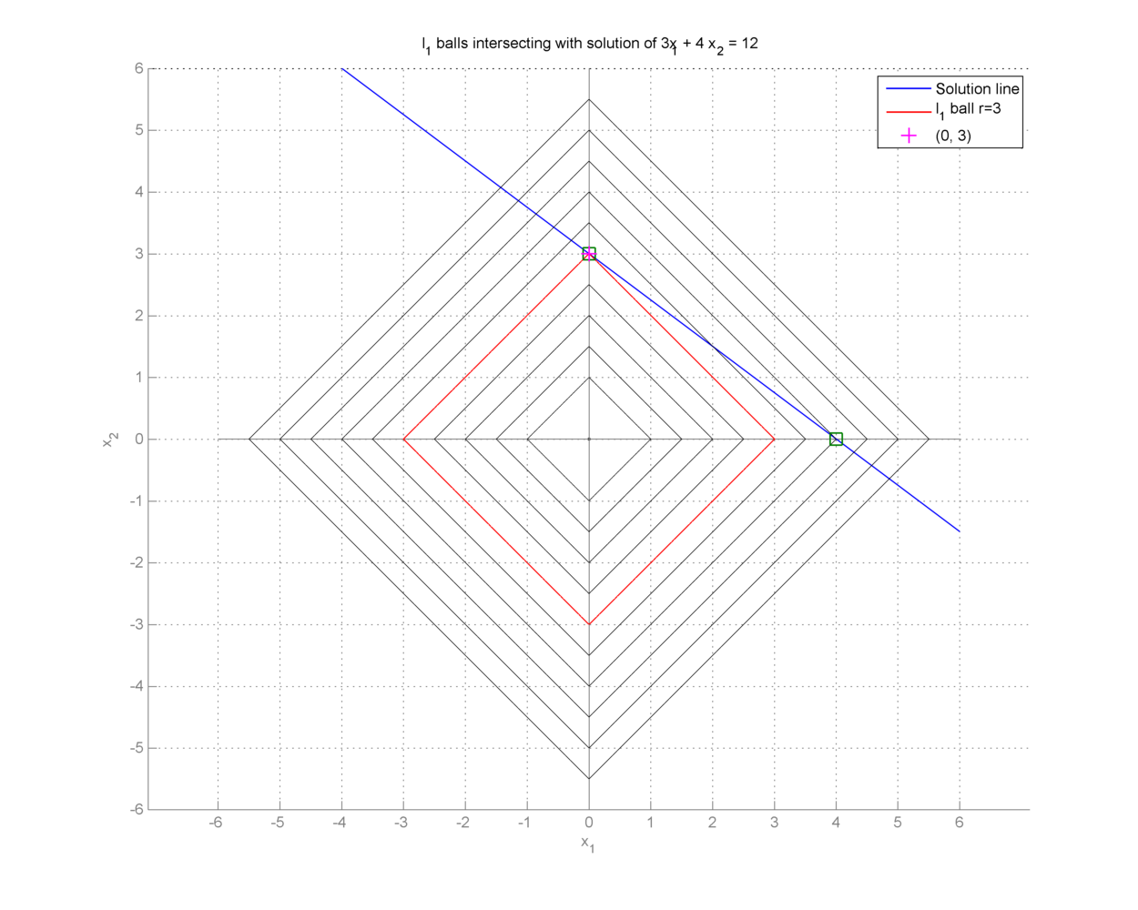
As we can see from the figure the minimum \(l_1\) norm solution is given by \((x_1,x_2) = (0,3)\).

It is interesting to note that \(l_1\) norm solution promotes sparser solutions while \(l_2\) norm solution promotes solutions in which signal energy is distributed amongst all of its components.

It’s time to have a closer look at our cost function \(J(x) = \|x \|_1\). This function is convex yet not strictly convex.

Example:math:`\| x\|_1` is not strictly convex

Consider again \(x \in \RR^2\). For \(x \in \RR_+^2\) (the first quadrant),

\[\|x \|_1 = x_1 + x_2.\]

Hence for any \(c_1, c_2 \geq 0\) and \(x, y \in \RR_+^2\):

\[\|(c_1 x + c_2 y)\|_1 = (c_1 x + c_2 y)_1 + (c_1 x + c_2 y)_2 = c_1 \| x\|_1 + c_2 \| y \|_1.\]

Thus, \(l_1\)-norm is not strictly convex. Consequently, a unique solution may not exist for \(l_1\) norm minimization problem.

As an example consider the under-determined system

\[3 x_1 + 3 x_2 = 12.\]

We can easily visualize that the solution line will pass through points \((0,4)\) and \((4,0)\). Moreover, it will be clearly parallel with \(l_1\)-norm ball of radius \(4\) in the first quadrant. See again the figure above. This gives us infinitely possible solutions to the minimization problem.

We can still observe that

• These solutions are gathered in a small line segment that is bounded (a bounded convex set) and
• There exist two solutions \((4,0)\) and \((0,4)\) amongst these solutions which have only 1 non-zero component.

For the \(l_1\) norm minimization problem since \(J(x)\) is not strictly convex, hence a unique solution may not be guaranteed. In specific cases, there may be infinitely many solutions. Yet what we can claim is begin{itemize} item these solutions are gathered in a set that is bounded and convex, and item among these solutions, there exists at least one solution with at most \(M\) non-zeros (as the number of constraints in \(\Phi x = y\)). end{itemize} todo{Provide reference to the claim that solution set is convex and bounded} todo{Show that at least one solution exists with \(M\) sparsity level}

Theorem

Let \(S\) denote the solution set of \(l_1\) norm minimization problem. \(S\) contains at least one solution \(\widehat{x}\) with \(\| \widehat{x} \|_0 = M\).

Proof

We have

• \(S\) is convex and bounded.
• \(\Phi x^* = y \, \Forall x^* \in S\).
• Since \(\Phi \in \RR^{M \times N}\) is full rank and \(M < N\), hence \(\text{rank}(\Phi) = M\).

Let \(x^* \in S\) be an optimal solution with \(\| x^* \|_0 = L > M\).

Consider the \(L\) columns of \(\Phi\) which correspond to \(\supp(x^*)\).

Since \(L > M\) and \(\text{rank}(\Phi) = M\) hence these columns linearly dependent.

Thus there exists a vector \(h \in \RR^N\) with \(\supp(h) \subseteq \supp(x^*)\) such that

\[\Phi h = 0.\]

Note that since we are only considering those columns of \(\Phi\) which correspond to \(\supp(x)\), hence we require \(h_i = 0\) whenever \(x^*_i = 0\).

Consider a new vector

\[x = x^* + \epsilon h\]

where \(\epsilon\) is small enough such that every element in \(x\) has the same sign as \(x^*\).

As long as

\[|\epsilon| \leq \underset{i \in \supp(x^*)}{\min} \frac{|x^*_i|}{|h_i|} = \epsilon_0\]

such an \(x\) can be constructed.

Note that \(x_i = 0\) whenever \(x^*_i = 0\).

Clearly

\[\Phi x = \Phi (x^* + \epsilon h) = y + \epsilon 0 = y.\]

Thus \(x\) is a feasible solution to the problem (1) though it need not be an optimal solution.

But since \(x^*\) is optimal hence, we must assume that \(l_1\) norm of \(x\) is greater than or equal to the \(l_1\) norm of \(x^*\)

\[\|x \|_1 = \|x^* + \epsilon h \|_1 \geq \| x^* \|_1 \Forall |\epsilon| \leq \epsilon_0.\]

Now look at \(\|x \|_1\) as a function of \(\epsilon\) in the region \(|\epsilon| \leq \epsilon_0\).

In this region, \(l_1\) function is continuous and differentiable since all vectors \(x^* + \epsilon h\) have the same sign pattern. If we define \(y^* = | x^* |\) (the vector of absolute values), then

\[\| x^* \|_1 = \| y^* \|_1 = \sum_{i=1}^N y^*_i.\]

Since the sign patterns don’t change, hence

\[|x_i| = |x^*_i + \epsilon h_i | = y^*_i + \epsilon h_i \sgn(x^*_i).\]

Thus

\[\begin{split}\begin{aligned} \|x \|_1 &= \sum_{i=1}^N |x_i| \\ &= \sum_{i=1}^N \left (y^*_i + \epsilon h_i \sgn(x^*_i) \right) \\ &= \| x^* \|_1 + \epsilon \sum_{i=1}^N h_i \sgn(x^*_i)\\ &= \| x^* \|_1 + \epsilon h^T \sgn(x^*). \end{aligned}\end{split}\]

The quantity \(h^T \sgn(x^*)\) is a constant. The inequality \(\|x \|_1 \geq \| x^* \|_1\) applies to both positive and negative values of \(\epsilon\) in the region \(|\epsilon | \leq \epsilon_0\). This is possible only when inequality is in fact an equality.

This implies that the addition / subtraction of \(\epsilon h\) under these conditions does not change the \(l_1\) length of the solution. Thus, \(x \in S\) is also an optimal solution.

This can happen only if

\[h^T \sgn(x^*) = 0.\]

We now wish to tune \(\epsilon\) such that one entry in \(x^*\) gets nulled while keeping the solutions \(l_1\) length.

We choose \(i\) corresponding to \(\epsilon_0\) (defined above) and pick

\[\epsilon = \frac{-x^*_i}{h_i}.\]

Clearly for the corresponding

\[x = x^* + \epsilon h\]

the \(i\)-th entry is nulled while others keep their sign and the \(l_1\) norm is also preserved. Thus, we have got a new optimal solution with \(L-1\) non-zeros at the most. It is possible that more than 1 entries get nulled this operation.

We can repeat this procedure till we are left with \(M\) non-zero elements.

Beyond this we may not proceed since \(\text{rank}(\Phi) = M\) hence we cannot say that corresponding columns of \(\Phi\) are linearly dependent.

We thus note that \(l_1\) norm has a tendency to prefer sparse solutions. This is a well known and fundamental property of linear programming.

\(l_1\) norm minimization problem as a linear programming problem

We now show that \(l_1\) norm minimization problem in \(\RR^N\) is in fact a linear programming problem.

Recalling the problem:

(1)\[\begin{split}\begin{aligned} & \underset{x \in \RR^N}{\text{minimize}} & & \| x \|_1 \\ & \text{subject to} & & y = \Phi x. \end{aligned}\end{split}\]

Let us write \(x\) as \(u - v\) where \(u, v \in \RR^N\) are both non-negative vectors such that \(u\) takes all positive entries in \(x\) while \(v\) takes all the negative entries in \(x\).

Example:math:`x = u - v`

Let

\[\]

x = (-1, 0 , 0 , 2, 0 , 0, 0, 4, 0, 0, -3, 0 , 0 , 0 , 0, 2 , 10).

Then

\[\]

u = (0, 0 , 0 , 2, 0 , 0, 0, 4, 0, 0, 0, 0 , 0 , 0 , 0, 2 , 10).

And

\[\]

v = (1, 0 , 0 , 0, 0 , 0, 0, 0, 0, 0, 3, 0 , 0 , 0 , 0, 0 , 0).

Clearly \(x = u - v\).

We note here that by definition

\[\supp(u) \cap \supp(v) = \EmptySet\]

i.e. support of \(u\) and \(v\) do not overlap.

We now construct a vector

\[\begin{split}z = \begin{bmatrix} u \\ v \end{bmatrix} \in \RR^{2N}.\end{split}\]

We can now verify that

\[\| x \|_1 = \|u\|_1 + \| v \|_1 = 1^T z.\]

And

\[\begin{split}\Phi x = \Phi (u - v) = \Phi u - \Phi v = \begin{bmatrix} \Phi & -\Phi \end{bmatrix} \begin{bmatrix} u \\ v \end{bmatrix} = \begin{bmatrix} \Phi & -\Phi \end{bmatrix} z\end{split}\]

where \(z \succeq 0\).

Hence the optimization problem (1) can be recast as

(2)\[\begin{split}\begin{aligned} & \underset{z \in \RR^{2N}}{\text{minimize}} & & 1^T z \\ & \text{subject to} & & \begin{bmatrix} \Phi & -\Phi \end{bmatrix} z = y\\ & \text{and} & & z \succeq 0. \end{aligned}\end{split}\]

This optimization problem has the classic Linear Programming structure since the objective function is affine as well as constraints are affine.

Let \(z^* =\begin{bmatrix} u^* \\ v^* \end{bmatrix}\) be an optimal solution to the problem (2).

In order to show that the two optimization problems are equivalent, we need to verify that our assumption about the decomposition of \(x\) into positive entries in \(u\) and negative entries in \(v\) is indeed satisfied by the optimal solution \(u^*\) and \(v^*\). i.e. support of \(u^*\) and \(v^*\) do not overlap.

Since \(z \succeq 0\) hence \(\langle u^* , v^* \rangle \geq 0\). If support of \(u^*\) and \(v^*\) don’t overlap, then we have \(\langle u^* , v^* \rangle = 0\). And if they overlap then \(\langle u^* , v^* \rangle > 0\).

Now for the sake of contradiction, let us assume that support of \(u^*\) and \(v^*\) do overlap for the optimal solution \(z^*\).

Let \(k\) be one of the indices at which both \(u_k \neq 0\) and \(v_k \neq 0\). Since \(z \succeq 0\), hence \(u_k > 0\) and \(v_k > 0\).

Without loss of generality let us assume that \(u_k > v_k > 0\).

In the equality constraint

\[\begin{split}\begin{bmatrix} \Phi & -\Phi \end{bmatrix} \begin{bmatrix} u \\ v \end{bmatrix} = y\end{split}\]

Both of these coefficients multiply the same column of \(\Phi\) with opposite signs giving us a term

\[\phi_k (u_k - v_k).\]

Now if we replace the two entries in \(z^*\) by

\[u_k' = u_k - v_k\]

and

\[v_k' = 0\]

to obtain an new vector \(z'\), we see that there is no impact in the equality constraint

\[\begin{bmatrix} \Phi & -\Phi \end{bmatrix} z = y.\]

Also the positivity constraint

\[z \succeq 0\]

is satisfied. This means that \(z'\) is a feasible solution.

On the other hand the objective function \(1^T z\) value reduces by \(2 v_k\) for \(z'\). This contradicts our assumption that \(z^*\) is the optimal solution.

Hence for the optimal solution of (2) we have

\[\supp(u^*) \cap \supp(v^*) = \EmptySet\]

thus

\[x^* = u^* - v^*\]

is indeed the desired solution for the optimization problem (1).