Dirac-DCT dictionary
This dictionary is suitable for real signals since both Dirac and DCT are totally real bases \(\in \RR^{N \times N}\).
The dictionary is obtained by combining the \(N \times N\) identity matrix (Dirac basis) with the \(N \times N\) DCT matrix for signals in \(\RR^N\).
Let \(\Psi_{\text{DCT}, N}\) denote the DCT matrix for \(\RR^N\). Let \(I_N\) denote the identity matrix for \(\RR^N\). Then
Let
The \(k\)-th column of \(\Psi_{\text{DCT}, N}\) is given by
with \(\Omega_k = \frac{1}{\sqrt{2}}\) for \(k=1\) and \(\Omega_k = 1\) for \(2 \leq k \leq N\).
Note that for \(k=1\), the entries become
Thus, the \(l_2\) norm of \(\psi_1\) is 1. We can similarly verify the \(l_2\) norm of other columns also. They are all one.
The coherence of a two ortho basis where one basis is Dirac basis is given by the magnitude of the largest entry in the other basis. For \(\Psi_{\text{DCT}, N}\), the largest value is obtained when \(\Omega_k = 1\) and the \(\cos\) term evaluates to 1. Clearly,
The \(p\)-babel function for Dirac-DCT dictionary is given by
In particular, the standard babel function is given by
Hands-on with Dirac DCT dictionaries
We need to specify the dimension of the ambient space:
N = 256;
We are ready to construct the dictionary:
Phi = spx.dict.simple.dirac_dct_mtx(N);
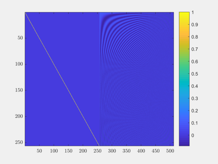
Let’s visualize the dictionary:
imagesc(Phi);
colorbar;
Measuring the coherence of the dictionary:
>> spx.dict.coherence(Phi)

ans =

    0.0884
We can cross-check with the theoretical estimate:
>> sqrt(2/N)

ans =

    0.0884
Let’s construct the babel function for this dictionary:
mu1 = spx.dict.babel(Phi);
We can plot it:
plot(mu1);
grid on;

We note that the babel function increases linearly for the initial part and saturates to a value of 16 afterwards.