Outline
In this chapter we develop initial concepts of sparse signal models.
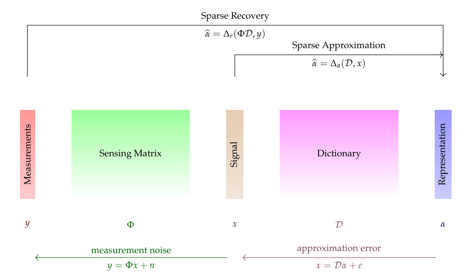
A bird’s eye view of the sparse representations and compressive sensing framework. Signals (like speech, images, etc.) reside in a signal space \(\RR^N\). Analytical or trained dictionaries can be constructed such that the signals can have a sparse representation in such dictionaries. These sparse representations reside in a representation space \(\RR^D\). A sparse approximation algorithm \(\Delta_a\) can construct a representation \(\alpha\) for a signal \(x\) in the dictionary \(\DDD\). The approximation error is \(e\). A small number of \(M\) random measurements are sufficient to capture all the information in \(x\). The sensing process \(y = \Phi x + n\) constructs the measurement vector \(y \in \RR^M\) for a given signal where \(n\) is the measurement noise. In order to get \(x\) from \(y\), we first need to recover the sparse representation \(\alpha\) using the sparse recovery algorithm \(\Delta_r\). Then \(x \approx \DDD \alpha\).
We begin our study with a review of solutions of under-determined systems. We build a case for solutions which promote sparsity.
We show that although the real life signals may not be sparse yet they are compressible and can be approximated with sparse signals.
We then review orthonormal bases and explain the inadequacy of those bases in exploiting the sparsity in many signals of interest. We develop an example of Dirac Fourier basis as a two ortho basis and demonstrate how it can better exploit signal sparsity compared to Dirac basis and Fourier basis individually.
We follow this with a general discussion of redundant signal dictionaries. We show how they can be used to create sparse and redundant signal representations.
We study various properties of signal dictionaries which are useful in characterizing the capabilities of a signal dictionary in exploiting signal sparsity.
In this chapter, our signals of interest will typically lie in the finite \(N\)-dimensional complex vector space \(\CC^N\). Sometimes we will restrict our attention to the \(N\) dimensional Euclidean space to simplify discussion.
We will be concerned with different representations of our signals of interest in \(\CC^D\) where \(D \geq N\). This aspect will become clearer as we go along in this chapter.
Sparsity
We quickly define the notion of sparsity in a signal.
We recall the definition of \(l_0\)-“norm” (don’t forget the quotes) of \(x \in \CC^N\) given by
where \(\supp(x) = \{ i : x_i \neq 0\}\) denotes the support of \(x\).
Informally we say that a signal \(x \in \CC^N\) is term{sparse} if \(\| x \|_0 \ll N\). index{Sparse signal}
More generally if \(x =\DDD \alpha\) where \(\DDD \in \CC^{N \times D}\) with \(D > N\) is some signal dictionary (to be formally defined later), then \(x\) is sparse in dictionary \(\DDD\) if \(\| \alpha \|_0 \ll D\).
Sometimes we simply say that \(x\) is \(K\)-sparse if \(\| x \|_0 \leq K\) where \(K < N\). We do not specifically require that \(K \ll N\).
An even more general definition of sparsity is the degrees of freedom a signal may have.
As an example consider all points on the surface of a unit sphere in \(\RR^N\). For every point \(x\) belonging to the surface \(|x|_2 = 1\). Thus if we choose the values of \(N-1\) components of \(x\) then the value of the remaining component is automatically fixed. Thus the number of degrees of freedom \(x\) has on the surface of the unit sphere in \(\RR^N\) is actually \(N-1\). Such a surface represents a manifold in the ambient Euclidean space. Of special interest are low dimensional manifolds where the number of degrees of freedom \(K \ll N\).