Synthetic Data Generation

Random Subspaces

Subspace clustering is focused on segmenting data which fall in different subspaces where subspaces are either independent or disjoint with each other and they are sufficiently oriented away from each other.

For testing algorithms, it is useful to pick random subspaces of an ambient signal space and then draw data points within these subspaces.

A way to pick a random subspace is to pick a basis for the subspace. Then, all the linear combinations of the basis elements fall in the subspace and the basis elements span every vector in the said random subspace.

Let’s pick a random plane in the 3-Dimensional space:

>> basis = orth(randn(3, 2))
basis =

   -0.2634    0.6981
   -0.5459   -0.6769
    0.7954   -0.2334

What we are doing is we are constructing a 3x2 Gaussian random matrix and orthogonalizing its columns. With probability 1, the Gaussian random matrix is full rank. Hence, this is a safe way of choosing a basis for a random plane.

We can verify that the basis is indeed orthogonal:

>> basis'*basis
ans =

    1.0000         0
         0    1.0000

Visualizing Subspaces

It is possible to visualize 2D subspaces in 3D space.

Let’s pick one subspace:

rng(10);
A = orth(randn(3, 2))

Identify its basis vectors:

e1 = A(:, 1);
e2 = A(:, 2);

Identify the corner points of a square around its basis vectors:

corners = [e1+e2, e2-e1, -e1-e2, -e2+e1];

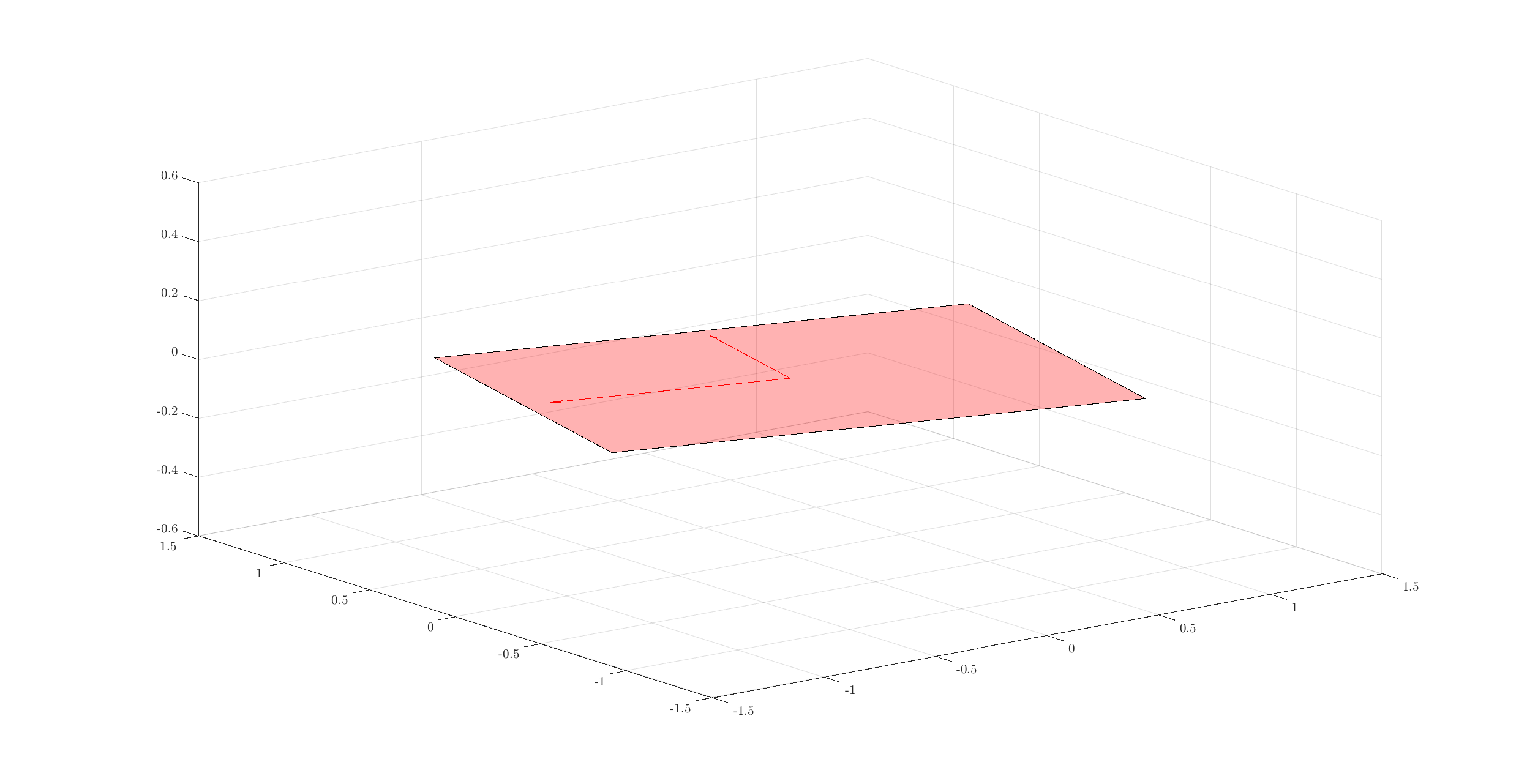
Visualize it:

fill3(corners(1,:),corners(2,:),corners(3,:),'r');
grid on;
hold on;
alpha(0.3);

Add the arrows of basis vectors from origin:

quiver3(0, 0, 0, e1(1), e1(2), e1(3), 'color', 'r');
quiver3(0, 0, 0, e2(1), e2(2), e2(3), 'color', 'r');

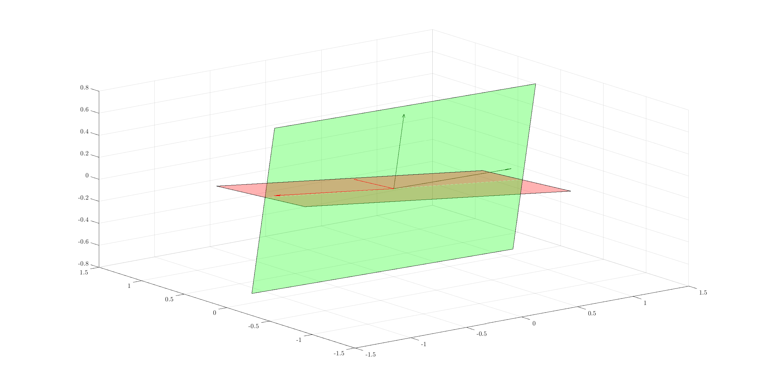
Let’s add one more basis:

B = orth(randn(3, 2));
e1 = B(:, 1);
e2 = B(:, 2);
corners = [e1+e2, e2-e1, -e1-e2, -e2+e1];
fill3(corners(1,:),corners(2,:),corners(3,:),'g');
alpha(0.3);
quiver3(0, 0, 0, e1(1), e1(2), e1(3), 'color', spx.graphics.rgb('DarkGreen'));
quiver3(0, 0, 0, e2(1), e2(2), e2(3), 'color', spx.graphics.rgb('DarkGreen'));

Multiple Subspaces

sparse-plex provides a way to draw multiple random subspaces of a given dimension from an ambient space.

Let’s pick the dimension of the ambient space:

M = 10;

Let’s pick the dimension of subspaces:

D = 4;

Let’s pick the number of subspaces to be drawn:

K = 2;

Let’s draw the bases for each random subspace:

import spx.data.synthetic.subspaces.random_subspaces;
bases = random_subspaces(M, K, D);

The result bases is a cell array containing the orthogonal basis for each subspace:

>> bases{1}

ans =

   -0.1178   -0.1432    0.0438   -0.0100
    0.1311   -0.0110   -0.4409    0.1758
    0.5198   -0.6404    0.0422   -0.3980
    0.5211   -0.0172   -0.2929    0.6334
   -0.2253   -0.1194   -0.2797    0.0920
    0.4695    0.1059    0.5408    0.1396
    0.1919    0.0765   -0.1441   -0.3519
    0.0940    0.0145   -0.4542   -0.4078
    0.3209    0.6274   -0.2325   -0.2118
   -0.0855   -0.3791   -0.2537    0.2153

>> bases{2}

ans =

    0.4784   -0.0579   -0.4213   -0.0206
    0.1213   -0.0591    0.3498    0.2351
    0.3077   -0.2110    0.2573    0.0042
   -0.5581   -0.5284    0.0988   -0.1403
    0.1128    0.5914    0.2518   -0.1872
   -0.1804   -0.0095    0.0707   -0.1351
   -0.0728    0.2774   -0.2063    0.3801
   -0.4417    0.3878    0.2071    0.4004
    0.0695   -0.2496   -0.1836    0.7344
    0.3158   -0.1732    0.6608    0.1647

Verify orthogonality:

>> Psi = bases{1}
>> Psi' * Psi

ans =

    1.0000   -0.0000   -0.0000   -0.0000
   -0.0000    1.0000    0.0000    0.0000
   -0.0000    0.0000    1.0000   -0.0000
   -0.0000    0.0000   -0.0000    1.0000

Principal Angles

If \(\UUU\) and \(\VVV\) are two linear subspaces of \(\RR^M\), then the smallest principal angle between them denoted by \(\theta\) is defined as [BjorckG73]

\[\cos \theta = \underset{u \in \UUU, v \in \VVV}{\max} \frac{u^T v}{\| u \|_2 \| v \|_2}.\]

For the functions provided in sparse-plex for measuring principal angles, see Hands on with Principal Angles.

Uniformly Distributed Points in Space

If we wish to generate points uniformly distributed on unit sphere, we have to follow the following two step procedure:

1. Generate independent standard Gaussian random vectors.
2. Normalize their lengths.

Here is an example.

Let ambient space dimension be:

>> M = 4;

Let number of points to be generated by:

>> S = 6;

Let’s generate the Gaussian random vectors:

>> X = randn(M, S)

X =

   -0.6568   -0.2926   -0.4930    0.6113    1.8045    0.6001
   -1.4814   -0.5408   -0.1807    0.1093   -0.7231    0.5939
    0.1555   -0.3086    0.0458    1.8140    0.5265   -2.1860
    0.8186   -1.0966   -0.0638    0.3120   -0.2603   -1.3270

Let’s normalize them:

>> X = spx.norm.normalize_l2(X)

X =

   -0.3605   -0.2260   -0.9286    0.3147    0.8886    0.2228
   -0.8130   -0.4177   -0.3404    0.0563   -0.3561    0.2205
    0.0853   -0.2384    0.0863    0.9338    0.2593   -0.8117
    0.4492   -0.8471   -0.1201    0.1606   -0.1282   -0.4928

Verify that they are indeed on the unit-sphere:

>> spx.norm.norms_l2_cw(X)

ans =

    1.0000    1.0000    1.0000    1.0000    1.0000    1.0000

We provide a reusable function to generate uniformly distributed points on unit sphere:

>> spx.data.synthetic.uniform(M, S)

ans =

   -0.6788    0.5450   -0.3194   -0.1977   -0.6098   -0.4051
    0.1893    0.3660    0.6441    0.2742    0.3803    0.1614
    0.6926   -0.7056   -0.0138   -0.0292   -0.0341   -0.6422
   -0.1540    0.2667    0.6949   -0.9407   -0.6946    0.6305

Uniformly Distributed Points in Subspaces

For subspace clustering purposes, individual vectors are usually normalized. They then fall onto the surface of the unit sphere of the subspace to which they belong.

For experimentation, it is useful to generate uniformly distributed points on the unit sphere of a random subspace.

It is actually very easy to do. Let’s start with a simple example of a random 2D plane inside 3D space.

Let’s choose a random plane:

basis = orth(randn(3, 2));

Let’s choose coordinates of some points in this basis where the coordinates are Gaussian distributed:

num_points = 100;
coefficients = randn(2, num_points);

Let’s normalize the coefficients:

coefficients = spx.norm.normalize_l2(coefficients);

The coordinates of these points in the 3D space can be easily calculated now:

uniform_points = basis * coefficients;

Verify that these points are indeed on unit sphere:

>> max(abs(spx.norm.norms_l2_cw(uniform_points) - 1))

ans =

   4.4409e-16

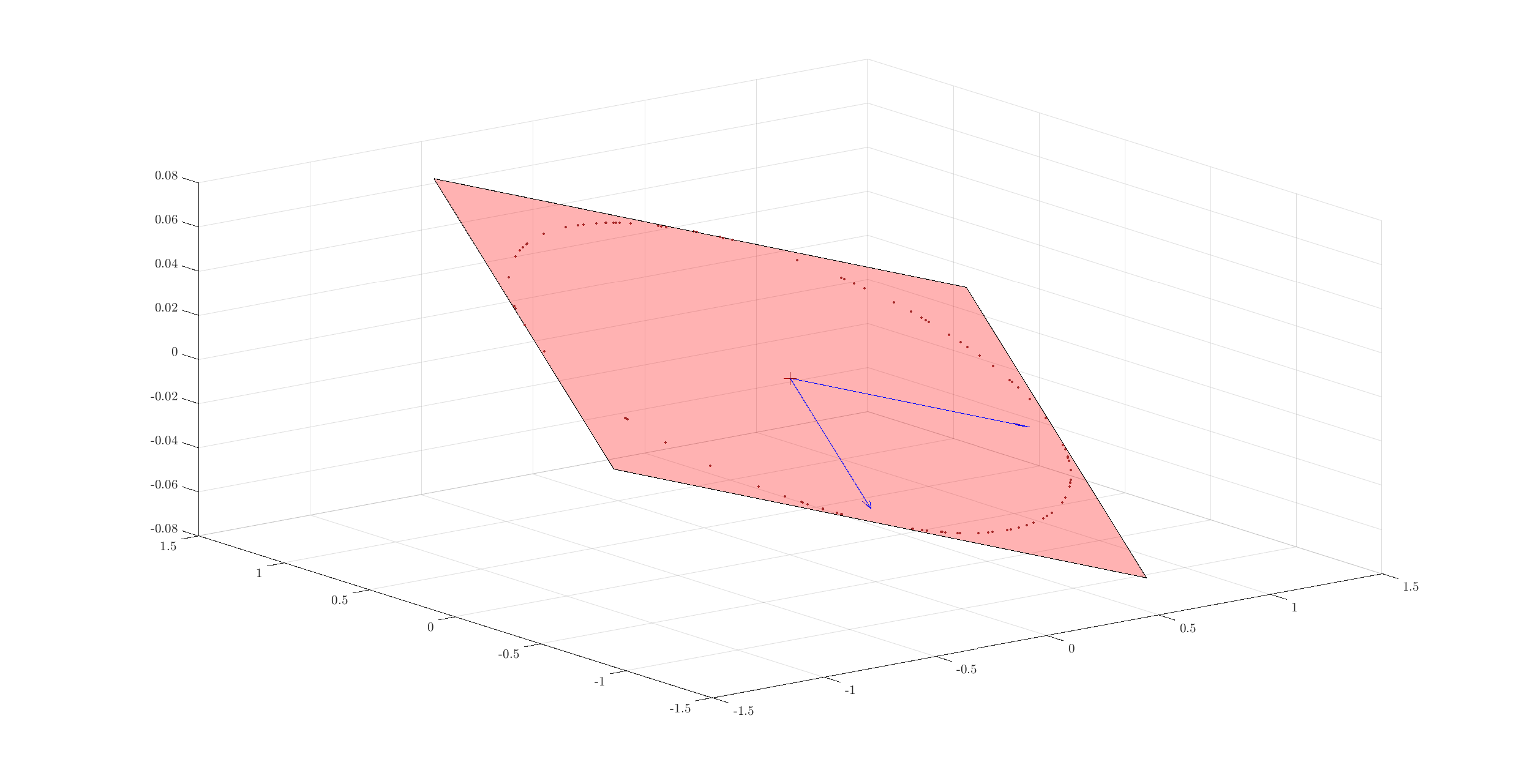
Time to visualize everything. First the plane:

e1 = basis(:, 1);
e2 = basis(:, 2);
corners = [e1+e2, e2-e1, -e1-e2, -e2+e1];
spx.graphics.figure.full_screen;
fill3(corners(1,:),corners(2,:),corners(3,:),'r');
grid on;
hold on;
alpha(0.3);

Then the unit vectors:

quiver3(0, 0, 0, e1(1), e1(2), e1(3), 'color', 'blue');
quiver3(0, 0, 0, e2(1), e2(2), e2(3), 'color', 'blue');

Finally the points:

x = uniform_points(1, :);
y = uniform_points(2, :);
z = uniform_points(3, :);
plot3(x, y, z, '.', 'color', spx.graphics.rgb('Brown') );

We might as well draw the origin too:

plot3(0, 0, 0, '+k', 'MarkerSize', 10, 'color', spx.graphics.rgb('DarkRed'));

Complete example code can be downloaded here.

Uniformly distributed points in multiple subspaces

We provide a useful function which can generate uniformly distributed points on one or more subspaces.

We first need to choose the bases for the subspaces for which we will draw uniformly distributed points. Here we will choose those bases randomly.

Ambient space dimension:

M = 10;

Number of subspaces:

K = 4;

Dimension of each subspace:

D = 5;

Bases for each subspace:

bases = spx.data.synthetic.subspaces.random_subspaces(M, K, D);

Now, let’s decide how many points do we need in each subspace:

cluster_sizes = [10 4 4 8];

Let’s generate uniformly distributed points in each subspace:

data_points = spx.data.synthetic.subspaces.uniform_points_on_subspaces(bases, cluster_sizes);

The returned value contains the data matrix containing the points and start and end indices for each cluster of points (for each subspace):

>> data_points

data_points =

  struct with fields:

                X: [10×26 double]
    start_indices: [1 11 15 19]
      end_indices: [10 14 18 26]

Let’s look at the start and end indices for each cluster:

>> data_points.start_indices

ans =

     1    11    15    19

>> data_points.end_indices

ans =

    10    14    18    26

Verify the size of the data matrix:

>> size(data_points.X)

ans =

    10    26

Let’s look at the data points for 2nd cluster:

>> data_points.X(:, data_points.start_indices(2):data_points.end_indices(2))

ans =

    0.0987    0.5278   -0.4014    0.2963
   -0.1793    0.0614    0.1551    0.2283
    0.4603    0.1510   -0.0926    0.0340
    0.3573   -0.1289    0.1654    0.4519
    0.1202   -0.0495    0.1382   -0.4503
   -0.1857   -0.6572   -0.1129   -0.3851
    0.4265    0.1540   -0.6315   -0.0117
   -0.4420    0.4131    0.0530    0.1565
    0.0262    0.1973   -0.2354    0.1153
   -0.4377   -0.1022    0.5385   -0.5155

Complete example code can be downloaded here.