Rademacher sensing matrices

In this section we collect several results related to Rademacher sensing matrices.

Definition

A Rademacher sensing matrix \(\Phi \in \RR^{M \times N}\) with \(M < N\) is constructed by drawing each entry \(\phi_{ij}\) independently from a Radamacher random distribution given by

(1)\[\PP_X(x) = \frac{1}{2}\delta\left(x-\frac{1}{\sqrt{M}}\right) + \frac{1}{2}\delta\left(x+\frac{1}{\sqrt{M}}\right).\]

Thus \(\phi_{ij}\) takes a value \(\pm \frac{1}{\sqrt{M}}\) with equal probability.

We can remove the scale factor \(\frac{1}{\sqrt{M}}\) out of the matrix \(\Phi\) writing

\[\Phi = \frac{1}{\sqrt{M}} \Chi\]

With that we can draw individual entries of \(\Chi\) from a simpler Rademacher distribution given by

(2)\[\PP_X(x) = \frac{1}{2}\delta(x-1) + \frac{1}{2}\delta(x + 1).\]

Thus entries in \(\Chi\) take values of \(\pm 1\) with equal probability.

This construction is useful since it allows us to implement the multiplication with \(\Phi\) in terms of just additions and subtractions. The scaling can be implemented towards the end in the signal processing chain.

We note that

\[\EE(\phi_{ij}) = 0.\]

\[\EE(\phi_{ij}^2) = \frac{1}{M}.\]

Actually we have a better result with

\[\phi_{ij}^2 = \frac{1}{M}.\]

We can write

\[\Phi = \begin{bmatrix} \phi_1 & \dots & \phi_N \end{bmatrix}\]

where \(\phi_j \in \RR^M\) is a Rademacher random vector with independent entries.

We note that

\[\EE (\| \phi_j \|_2^2) = \EE \left ( \sum_{i=1}^M \phi_{ij}^2 \right ) = \sum_{i=1}^M (\EE (\phi_{ij}^2)) = M \frac{1}{M} = 1.\]

Actually in this case we also have

\[\| \phi_j \|_2^2 = 1.\]

Thus the squared length of each of the columns in \(\Phi\) is \(1\) .

Lemma

Let \(z \in \RR^M\) be a Rademacher random vector with i.i.d entries \(z_i\) that take a value \(\pm \frac{1}{\sqrt{M}}\) with equal probability. Let \(u \in \RR^M\) be an arbitrary unit norm vector. Then

\[\PP \left ( | \langle z, u \rangle | > \epsilon \right ) \leq 2 \exp \left (- \epsilon^2 \frac{M}{2} \right ).\]

Representative values of this bound are plotted below.

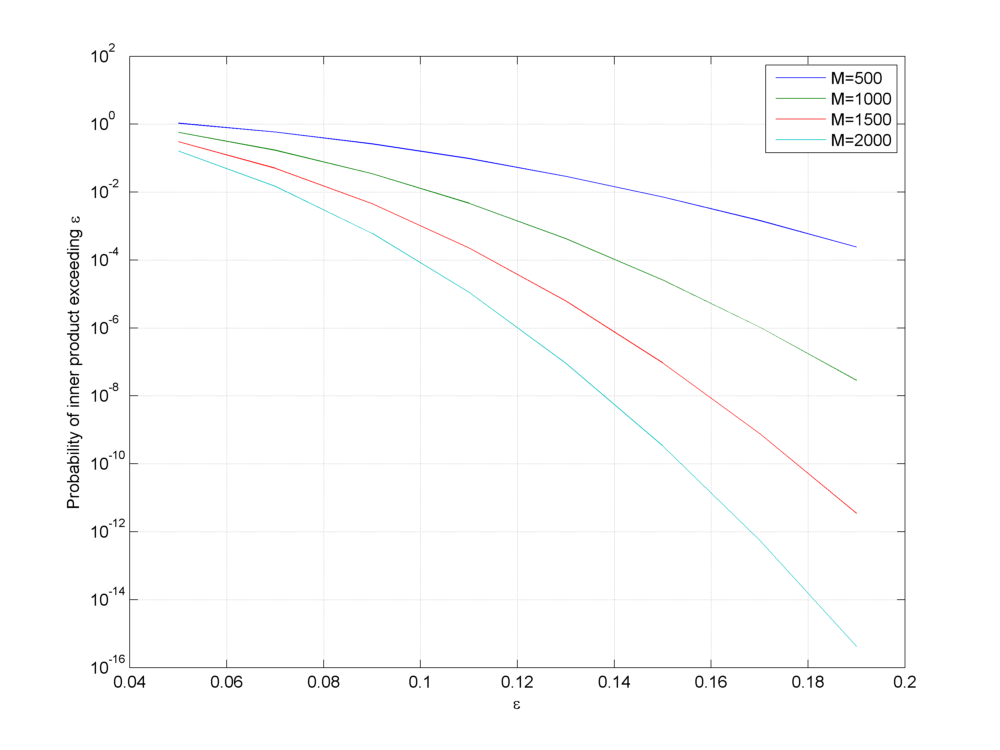
Tail bound for the probability of inner product of a Rademacher random vector with a unit norm vector

Proof

This can be proven using Hoeffding inequality. To be elaborated later.

A particular application of this lemma is when \(u\) itself is another (independently chosen) unit norm Rademacher random vector.

The lemma establishes that the probability of inner product of two independent unit norm Rademacher random vectors being large is very very small. In other words, independently chosen unit norm Rademacher random vectors are incoherent with high probability. This is a very useful result as we will see later in measurement of coherence of Rademacher sensing matrices.

Joint correlation

Columns of \(\Phi\) satisfy a joint correlation property ([TG07]) which is described in following lemma.

Lemma

Let \(\{u_k\}\) be a sequence of \(K\) vectors (where \(u_k \in \RR^M\) ) whose \(l_2\) norms do not exceed one. Independently choose \(z \in \RR^M\) to be a random vector with i.i.d. entries \(z_i\) that take a value \(\pm \frac{1}{\sqrt{M}}\) with equal probability. Then

\[\PP\left(\max_{k} | \langle z, u_k\rangle | \leq \epsilon \right) \geq 1 - 2 K \exp \left( - \epsilon^2 \frac{M}{2} \right).\]

Proof

Let us call \(\gamma = \max_{k} | \langle z, u_k\rangle |\) .

We note that if for any \(u_k\) , \(\| u_k \|_2 <1\) and we increase the length of \(u_k\) by scaling it, then \(\gamma\) will not decrease and hence \(\PP(\gamma \leq \epsilon)\) will not increase. Thus if we prove the bound for vectors \(u_k\) with \(\| u_k\|_2 = 1 \Forall 1 \leq k \leq K\) , it will be applicable for all \(u_k\) whose \(l_2\) norms do not exceed one. Hence we will assume that \(\| u_k \|_2 = 1\) .

From previous lemma we have

\[\PP \left ( | \langle z, u_k \rangle | > \epsilon \right ) \leq 2 \exp \left (- \epsilon^2 \frac{M}{2} \right ).\]

Now the event

\[\left \{ \max_{k} | \langle z, u_k\rangle | > \epsilon \right \} = \bigcup_{ k= 1}^K \{| \langle z, u_k\rangle | > \epsilon\}\]

i.e. if any of the inner products (absolute value) is greater than \(\epsilon\) then the maximum is greater.

We recall Boole’s inequality which states that

\[\PP \left(\bigcup_{i} A_i \right) \leq \sum_{i} \PP(A_i).\]

Thus

\[\PP\left(\max_{k} | \langle z, u_k\rangle | > \epsilon \right) \leq 2 K \exp \left (- \epsilon^2 \frac{M}{2} \right ).\]

This gives us

\[\begin{split}\begin{aligned} \PP\left(\max_{k} | \langle z, u_k\rangle | \leq \epsilon \right) &= 1 - \PP\left(\max_{k} | \langle z, u_k\rangle | > \epsilon \right) \\ &\geq 1 - 2 K \exp \left(- \epsilon^2 \frac{M}{2} \right). \end{aligned}\end{split}\]

Coherence of Rademacher sensing matrix

We show that coherence of Rademacher sensing matrix is fairly small with high probability (adapted from [TG07]).

Lemma

Fix \(\delta \in (0,1)\) . For an \(M \times N\) Rademacher sensing matrix \(\Phi\) as defined above, the coherence statistic

\[\mu \leq \sqrt{ \frac{4}{M} \ln \left( \frac{N}{\delta}\right)}\]

with probability exceeding \(1 - \delta\) .

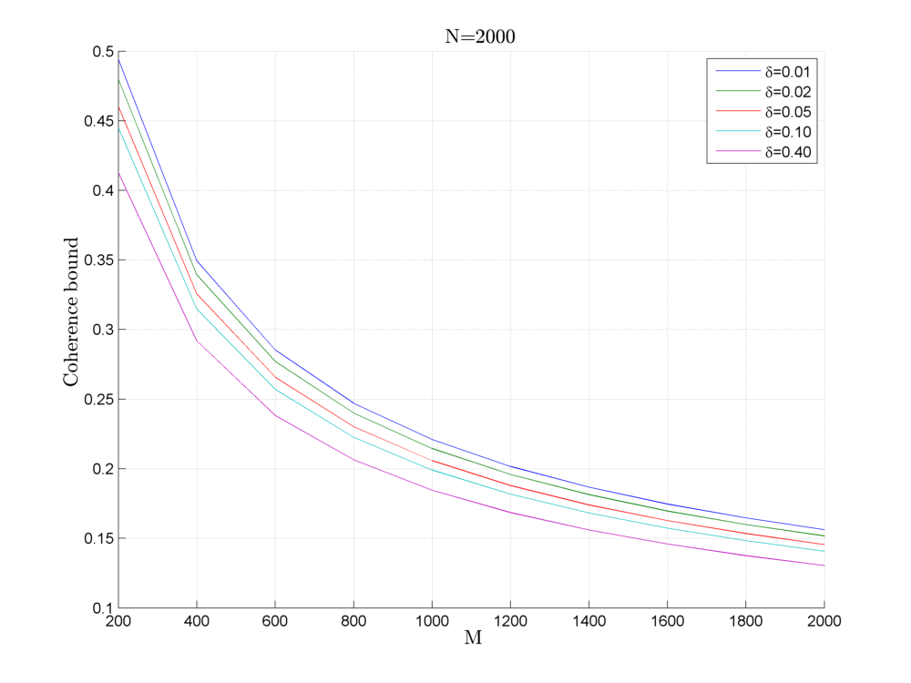
Coherence bounds for Rademacher sensing matrices

Proof

We recall the definition of coherence as

\[\mu = \underset{j \neq k}{\max} | \langle \phi_j, \phi_k \rangle | = \underset{j < k}{\max} | \langle \phi_j, \phi_k \rangle |.\]

Since \(\Phi\) is a Rademacher sensing matrix hence each column of \(\Phi\) is unit norm column. Consider some \(1 \leq j < k \leq N\) identifying columns \(\phi_j\) and \(\phi_k\) . We note that they are independent of each other. Thus from above we have

\[\PP \left ( |\langle \phi_j, \phi_k \rangle | > \epsilon \right ) \leq 2 \exp \left (- \epsilon^2 \frac{M}{2} \right ).\]

Now there are \(\frac{N(N-1)}{2}\) such pairs of \((j, k)\) . Hence by applying Boole’s inequality

\[\PP \left ( \underset{j < k} {\max} |\langle \phi_j, \phi_k \rangle | > \epsilon \right ) \leq 2 \frac{N(N-1)}{2} \exp \left (- \epsilon^2 \frac{M}{2} \right ) \leq N^2 \exp \left (- \epsilon^2 \frac{M}{2} \right ).\]

Thus, we have

\[\PP \left ( \mu > \epsilon \right )\leq N^2 \exp \left (- \epsilon^2 \frac{M}{2} \right ).\]

What we need to do now is to choose a suitable value of \(\epsilon\) so that the R.H.S. of this inequality is simplified.

We choose

\[\epsilon^2 = \frac{4}{M} \ln \left ( \frac{N}{\delta}\right ).\]

This gives us

\[\epsilon^2 \frac{M}{2} = 2 \ln \left ( \frac{N}{\delta}\right ) \implies \exp \left (- \epsilon^2 \frac{M}{2} \right ) = \left ( \frac{\delta}{N} \right)^2.\]

Putting back we get

\[\PP \left ( \mu > \epsilon \right )\leq N^2 \left ( \frac{\delta}{N} \right)^2 \leq \delta^2.\]

This justifies why we need \(\delta \in (0,1)\) .

Finally

\[\PP \left ( \mu \leq \sqrt{ \frac{4}{M} \ln \left( \frac{N}{\delta}\right)} \right ) = \PP (\mu \leq \epsilon) = 1 - \PP (\mu > \epsilon) > 1 - \delta^2\]

and

\[1 - \delta^2 > 1 - \delta\]

which completes the proof.