Examples
In this section we will look at several examples which can be modeled using sparse and redundant representations and measured using compressed sensing techniques.
Several examples in this section have been incorporated from Sparco [BFH+07] (a testing framework for sparse reconstruction).
Piecewise cubic polynomial signal
This example was discussed in [CR04]. Our signal of interest is a piecewise cubic polynomial signal as shown here.
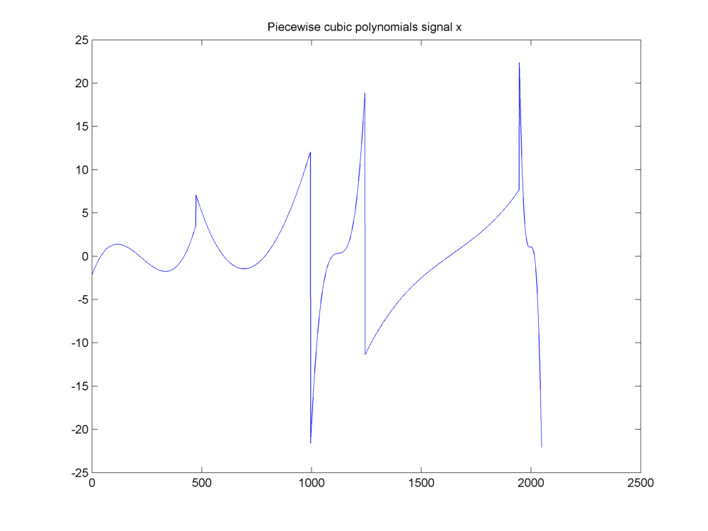
A piecewise cubic polynomials signal
It has a sparse representation in a wavelet basis.
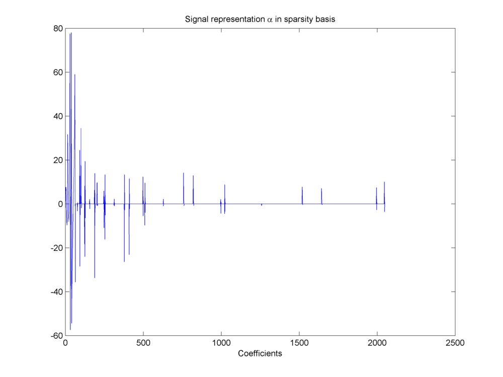
Sparse representation of signal in wavelet basis
We can sort the wavelet coefficients by magnitude and plot them in descending order to visualize how sparse the representation is.
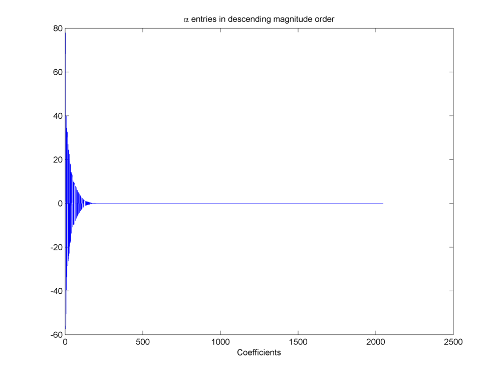
Wavelet coefficients sorted by magnitude
The chosen basis is a Daubechies wavelet basis \(\Psi\).
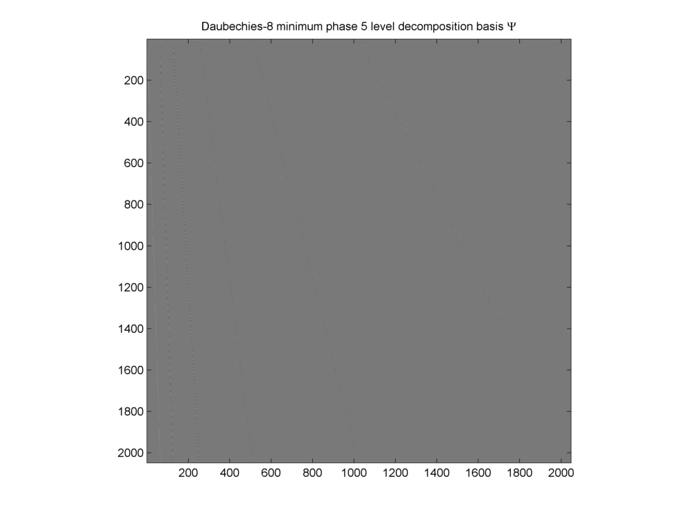
Daubechies-8 wavelet basis
A Gaussian random sensing matrix \(\Phi\) is used to generate the measurement vector \(y\)
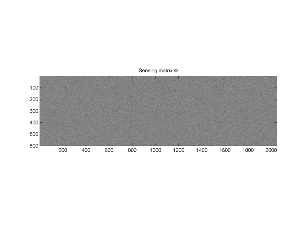
Gaussian sensing matrix \(\Phi\)
The measurements are shown here:
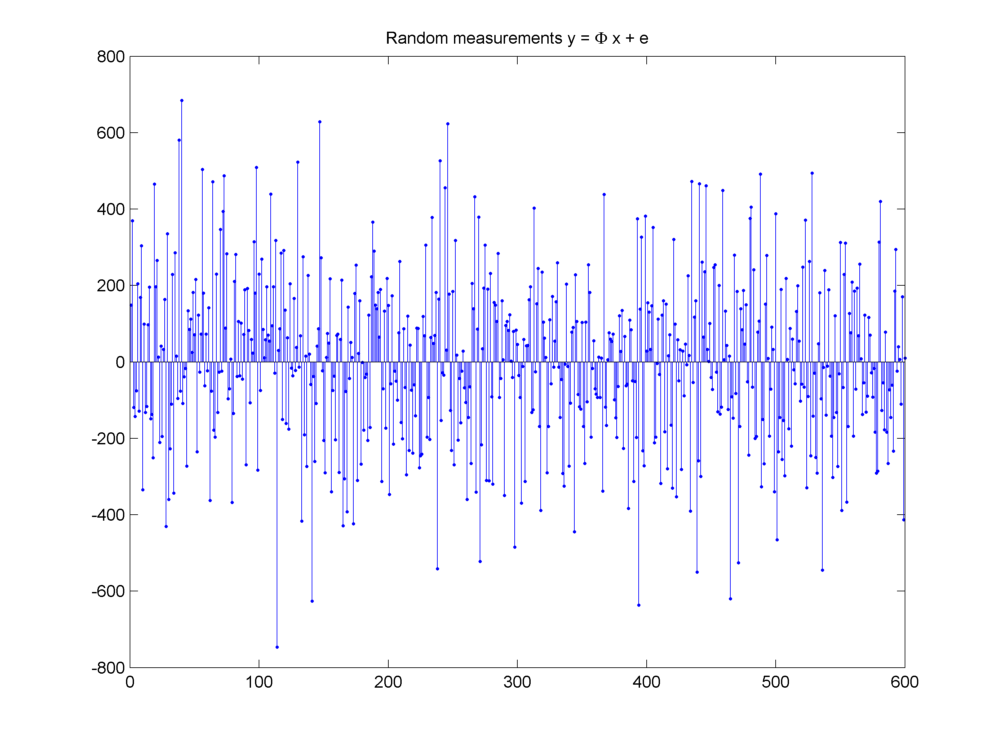
Measurement vector \(y = \Phi x + e\)
Finally the product of \(\Phi\) and \(\Psi\) given by \(\Phi \Psi\) will be used for actual recovery of sparse representation.
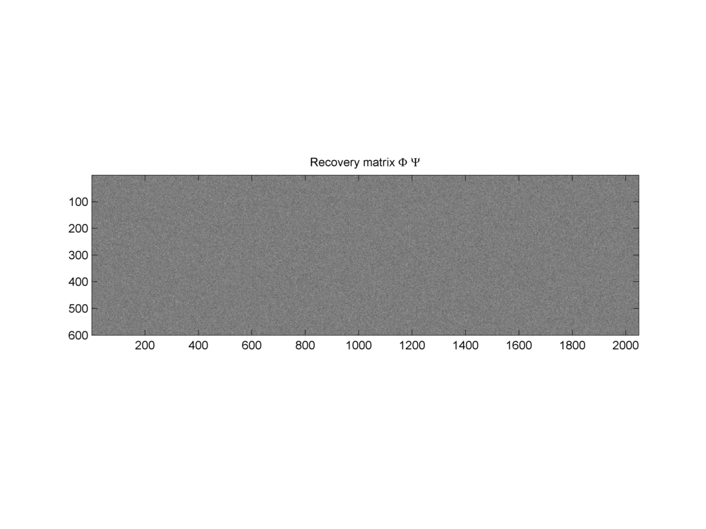
Recovery matrix \(\Phi \Psi\)
Fundamental equations are:
and
with \(x \in \RR^N\). In this example \(N = 2048\). \(\Psi\) is a complete dictionary of size \(N \times N\). Thus we have \(D = N\) and \(\alpha \in \RR^N\). \(\Phi \in \RR^{M \times N}\). In this example, the number of measurements \(M=600\). The measurement vector \(y \in \RR^M\). For this problem we chose \(e = 0\).
Sparse signal recovery problem is denoted as
where \(\widehat{\alpha}\) is a \(K\)-sparse approximation of \(\alpha\).
Closely examining the coefficients in \(\alpha\) we can note that \(\max(\alpha_i) = 78.0546\). Further if we put different thresholds over magnitudes of entries in \(\alpha\) we can find the number of coefficients higher than the threshold as listed in the table below. A choice of \(M = 600\) looks quite reasonable given the decay of entries in \(\alpha\).
| Threshold | Entries higher than threshold |
|---|---|
| 1 | 129 |
| 1E-1 | 173 |
| 1E-2 | 186 |
| 1E-4 | 197 |
| 1E-8 | 199 |
| 1E-12 | 200 |