Basic Operations
Essential operations in the implementation of a numerical algorithm are addition, multiplication, comparison, load and store. Numbers are stored in floating point representation. A dedicated floating point unit is available for performing arithmetic operations. These operations are known as floating point operations (flops). A typical update operation \(b \leftarrow b + x y\) (a.k.a. multiply and add) involves two flops (one floating point multiply and open floating point addition). Subtraction costs same as addition. A division is usually counted as 4 flops in HPC community as a more sophisticated procedure is invoked in the floating point arithmetic hardware. For our purposes, we will count division as single flop as it is a rare operation and doesn’t affect overall flop count asymptotically. A square root operation can take about 6 flops on typical CPU architectures, but [following [TBI97]], we will treat it as a single flop. We ignore the costs of load and store operations. We usually, also ignore costs of decision making operations and integer counters. We will also be treating real arithmetic as well as complex arithmetic costing same number of flops to maintain ease of analysis.
Let \(x, y \in \RR^n\) be two vectors, then their inner product is computed as
This involves \(n\) multiplications and \(n-1\) additions. Total operation count is \(2n - 1\) flops. If we implement this as a sequence of multiply and add operation starting with \(0\), then this will take \(2n\) flops. We will use this simpler expression. Addition and subtraction of \(x\) and \(y\) takes \(n\) flops. Scalar multiplication takes \(n\) flops.
Multiplication
Let \(A \in \RR^{m \times n}\) be a real matrix and \(x \in \RR^n\) be a vector. Then \(y = A x \in \RR^m\) is their matrix-vector product. A straight-forward implementation consists of taking inner product of each row of \(A\) with \(x\). Each inner product costs \(2n\) flops. There are \(m\) such inner products computed. Total operation count is \(2mn\). When two matrices \(A \in \RR^{m \times n}\) and \(B \in \RR^{n \times p}\) are multiplied, the operation count is \(2mnp\).
There are specialized matrix-matrix multiplication algorithms which can reduce the flop count, but we would be content with this result. If \(A\) has a certain structure [e.g. Fourier Transform], then specialized algorithms may compute the product much faster. We will not be concerned with this at the moment. Also, partitioning of a matrix into blocks and using block versions of fundamental matrix operations helps a lot in improving the memory traffic and can significantly improve the performance of the algorithm on real computers, but this doesn’t affect the flop count and we won’t burden ourselves with these details.
If \(A\) is diagonal (with \(m=n\)), then \(Ax\) can be computed in \(n\) flops. If \(A\) is lower triangular (with \(m=n\)), then \(Ax\) can be computed in \(n(n+1)\) flops. Here is a quick way to compute \((I + uv^T)x\): Compute \(c = v^T x\) (\(2n\) flops), then compute \(w = c u\) (\(n\) flops), then compute \(w + x\) (\(n\) flops). The total is \(4n\) flops.
The Gram Matrix \(G = A^T A\) (for \(A \in \RR^{m \times n}\)) is symmetric of size \(n \times n\). We need to calculate only the upper triangular part and we can fill the lower triangular part easily. Each row vector of \(A^T\) and column vector of \(A\) belong to \(\RR^{m}\). Their inner product takes \(2m\) flops. We need to compute \(n(n+1)/2\) such inner products. The total flop count is \(mn(n+1) \approx mn^2\). Similarly, the frame operator \(AA^T\) is symmetric requiring \(nm(m+1) \approx nm^2\) flops.
Squared norm of a vector \(\| x \|_2^2 = \langle x, x \rangle\) can be computed in \(2n-1\) flops. Norm can be computed in \(2n\) flops.
Elementary row operations
There are a few memory operations for which we need to assign flop counts. Setting a vector \(x \in \RR^n\) to zero (or any constant value) will take \(n\) flops. Swapping two rows of a matrix \(A\) (with \(n\) columns) takes \(3n\) flops.
Scaling a row of \(A\) takes \(n\) flops. Scaling a row and adding to another row takes \(2n\) flops.
Back and forward substitution
Given an upper triangular matrix \(L \in \RR^{n \times n}\), solving the equation \(L x = b\) takes \(n^2\) flops. This can be easily proved by induction. The case for \(n=1\) is trivial (requiring 1 division). Assume that the flop count is valid for \(1\dots n-1\). For \(n \times n\) matrix \(L\), let the top most row equation be
where \(x_2 \dots x_n\) are already determined in \((n-1)^2\) flops. Solving for \(x_1\) requires \(2n -3 + 1 + 1= 2n - 1\) flops. The total is \((n-1)^2 + 2n -1 = n^2\). Flop count for forward substitution is also \(n^2\).
Gaussian elimination
Let \(A \in \RR^{n \times n}\) be a full rank matrix and let us look at the Gaussian elimination process in solving the equation \(A x = y\) for a given \(y\) and unknown \(x\). As the pivot column shifts in Gaussian elimination process, the number of columns involved keeps reducing. The first pivot is \(a_{11}\). Computing its inverse takes 4 flops. For \(i\)-th row beneath the first row, computing \(a_{11} / a_{i1}\) takes 4 flops, scaling the row with this value takes \(n\) flops, and subtracting 1st from from this takes \(n\) flops. Total flop count is \((2n+1)\) flops. We repeat the same for \((n-1)\) rows. Total flop count is \((2n+1)(n-1)\). For \(i\)-th pivot from \(i\)-th row, the number of columns involved is \(n-i+1\). Number of rows below it is \(n-i\). Flop count of zeroing out entries below the pivot is \((2(n-i+1)+1)(n-i)\). Summing over \(1\) to \(n\), we obtain:
For a \(2\times 2\) matrix, this is 5 flops. For a \(3\times 3\) matrix, this is \(19\) flops. Actually, substituting \(n-i+1\) by \(k\), we can rewrite the sum as:
Additional \(n^2\) flops are required for back substitution part.
QR factorization
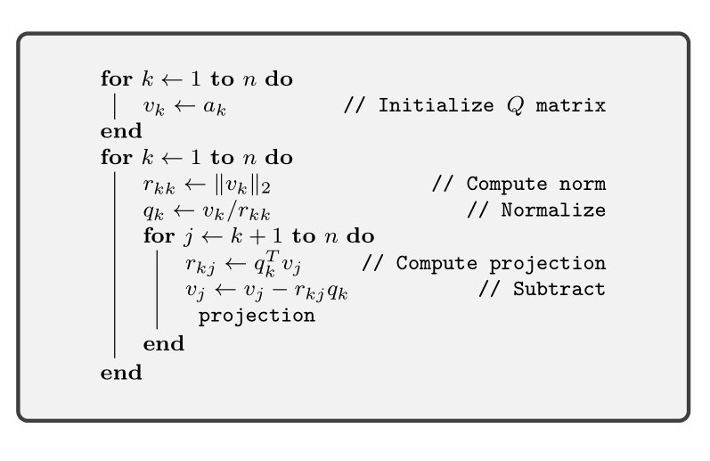
We factorize a full column rank matrix \(A \in \RR^{m \times n}\) as \(A = QR\) where \(Q \in \RR^{m \times n}\) is an orthogonal matrix \(Q^TQ = I\) and \(R \in \RR^{n \times n}\) is an upper triangular matrix. This can be computed in \(2mn^2\) flops using Modified Gram-Schmidt algorithm presented in here.
\caption{Modified Gram-Schmidt Algorithm}

\footnotesize
\SetAlgoLined
\For{:math:`k \leftarrow 1` \KwTo :math:`n`}{
    :math:`v_k \leftarrow a_k`\tcp*{Initialize :math:`Q` matrix}
}
\For{:math:`k \leftarrow 1` \KwTo :math:`n`}{
    :math:`r_{kk} \leftarrow \| v_k \|_2`\tcp*{Compute norm}
    :math:`q_k \leftarrow v_k / r_{kk}` \tcp*{Normalize}
    \For{:math:`j \leftarrow k+1` \KwTo :math:`n`} {
        :math:`r_{kj} \leftarrow q_k^T v_j` \tcp*{Compute projection}
        :math:`v_j \leftarrow v_j - r_{kj} q_k` \tcp*{Subtract projection}
    }
}
Most of the time of the algorithm is spent in the inner loop on \(j\). Projection of \(v_j\) on \(q_k\) is computed in \(2m-1\) flops. It is subtracted from \(v_j\) in \(2m\) flops. Projection of \(q_k\) is subtracted from remaining \((n-k)\) vectors requiring \((n-k)(4m-1)\) flops. Summing over \(k\), we get:
Computing norm \(r_{kk}\) requires \(2m\) flops. Computing \(q_k\) requires \(m+1\) flops (1 inverse and \(m\) multiplications). These contribute \((3m+1)n\) flops for \(n\) columns. Initialization of \(Q\) matrix can be absorbed into the normalization step requiring no additional flops. Thus, the total flop count is \(\frac{3n}{2} + m n + 2mn^2 - \frac{n^2}{2} \approx 2mn^2\).
A variation of this algorithm is presented below. In this version \(Q\) and \(R\) matrices are computed column by column from \(A\) matrix. This allows for incremental update of \(QR\) factorization of \(A\) as more columns in \(A\) are added. This variation is very useful in efficient implementation of algorithms like Orthogonal Matching Pursuit.
Again, the inner loop requires \(4m-1\) flops. This loop is run \(k-1\) times. We have \(\sum_{k=1}^n (k-1)= \sum_{k=1}^n (n - k)\). Thus, flop counts are identical.
Least Squares
Standard least squares problem of minimizing the norm squared \(\| A x - b\|_2^2\) where \(A\) is a full column rank matrix, can be solved using various methods. Solution can be obtained by solving the normal equations \(A^T A x = A^T b\). Since the Gram matrix \(A^T A\) is symmetric, faster solutions than Gaussian elimination are applicable.
QR factorization
We write \(A = QR\). Then, an equivalent formulation of normal equations is \(R x = Q^T b\). The solution is obtained in 3 steps: a) Compute \(QR\) factorization of \(A\). b) Form \(d = Q^T b\). c) Solve \(R x = d\) by back substitution. Total cost for solution is \(2mn^2 + 2mn + n^2\) flops. We refrain from ignoring the lower order terms as we will be using incremental QR update based series of least squares problems in sequel.
Cholesky factorization
We calculate \(G = A^T A\). We then perform the Cholesky factorization of \(G = LL^T\). We compute \(d = A^T b\). We solve \(Lz = d\) by forward substitution. We solve \(L^T x = z\) by back substitution. Total flop count is approximately \(mn^2 + (1/3) n^3 + 2mn + n^2 + n^2\) flops. For large \(m, n\), the cost is approximately \(mn^2 + (1/3) n^3\). QR factorization is numerically more stable though Cholesky is faster. Cholesky factorization can be significantly faster if \(A\) is a sparse matrix. Otherwise QR factorization is the preferred approach.
Incremental QR factorization
Let us spend some time on looking at the QR based solution differently. Let us say that \(A = \begin{bmatrix} a_1 & a_2 & \dots & a_n \end{bmatrix}\). Let \(A_k\) be the submatrix consisting of first \(k\) columns of \(A\). Let the QR factorization of \(A_k\) be \(Q_k R_k\). Let \(x_k\) be the solution of the least squares problem of minimizing \(\| A_k x_k - b \|_2^2\). We form \(d_k = Q_k^T b\) and solve \(R_k x_k = d_k\) via back substitution.
Similarly, QR factorization of \(A_{k+1}\) is \(Q_{k+1} R_{k+1}\). We can write
\(k\) entries in the vector \(r_{k+1}\) are computed as per the loop in above. Computing and subtracting projection of \(a_{k+1}\) for each normalized column in \(Q_k\) requires \(4m-1\) flops. This loop is run \(k\) times. Computing norm and division requires \(3m+1\) flops. The whole QR update step requires \(k(4m-1) + 3m + 1\) flops. It is clear that the first \(k\) entries in \(d_{k+1}\) are identical to \(d_k\). We just need to compute the last entry as \(q_{k+1}^T b\) (requiring \(2m\) flops). Back substitution will require all \((k+1)^2\) flops. Total number of flops required for solving the \(k+1\)-th least squares problem is \(k(4m-1) + 3m + 1 + 2m + (k+1)^2\) flops. Summing over \(k=0\) to \(n-1\), we get
Compare this with the flop count for QR factorization based least squares solution for whole matrix \(A\): \(2mn^2 + 2mn + n^2\). Asymptotically (with \(n < m\)), this is close to \(2mn^2\), the operation count for solving the full least squares problem. This approach gives us a series of solutions with sacrificing much on computational complexity.