Basic CS Tutorial
This tutorial is based on examples\\ex_simple_compressed_sensing_demo.m.
In this tutorial we will:
- Create sparse signals (with Gaussian and bi-uniform distributed non-zero samples).
- Look at how to identify support of a signal.
- Construct a Gaussian sensing matrix.
- Visualize the sensing matrix.
- Compute random measurements on the sparse signal with the sensing matrix.
- Add measurement noise to the measurements.
- Recover the sparse vector
using following sparse recovery algorithms
- Matching Pursuit
- Orthogonal Matching Pursuit
- Basis Pursuit
- Measure the recovery error for different sparse recovery algorithms.
Basic setup:
% Signal space
N = 1000;
% Number of measurements
M = 200;
% Sparsity level
K = 8;
Choosing the support randomly:
Omega = randperm(N, K);
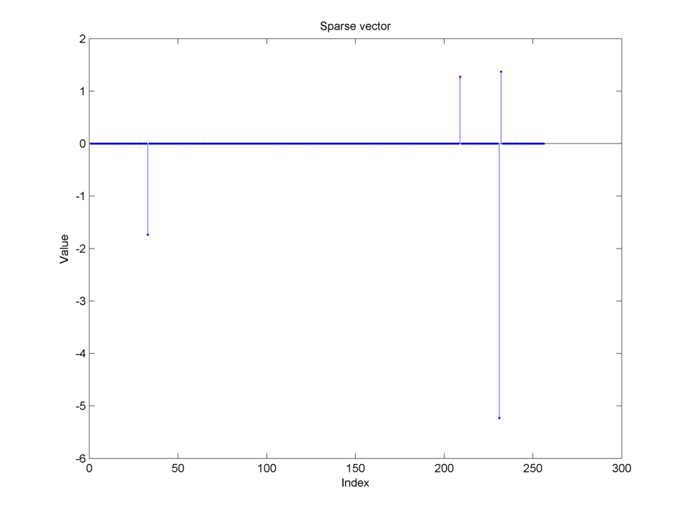
Constructing a sparse vector with Gaussian entries:
% Initializing a zero vector
x = zeros(N, 1);
% Filling it with non-zero Gaussian entries at specified support
x(Omega) = 4 * randn(K, 1);
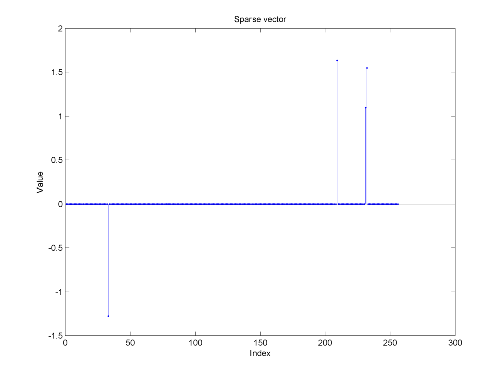
Constructing a bi-uniform sparse vector:
a = 1;
b = 2;
% unsigned magnitudes of non-zero entries
xm = a + (b-a).*rand(K, 1);
% Generate sign for non-zero entries randomly
sgn = sign(randn(K, 1));
% Combine sign and magnitude
x(Omega) = sgn .* xm;
Identifying support:
find(x ~= 0)'
% 98   127   277   544   630   815   905   911
Constructing a Gaussian sensing matrix:
Phi = randn(M, N);
% Make sure that variance is 1/sqrt(M)
Phi = Phi ./ sqrt(M);
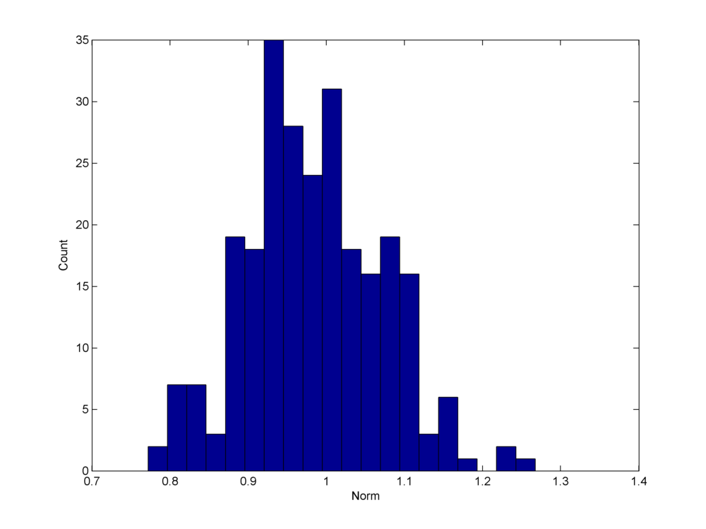
Computing norm of each column:
column_norms = sqrt(sum(Phi .* conj(Phi)));
Norm histogram
Constructing a Gaussian dictionary with normalized columns:
for i=1:N
    v = column_norms(i);
    % Scale it down
    Phi(:, i) = Phi(:, i) / v;
end
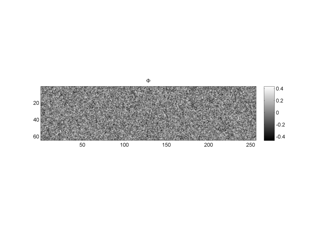
Visualizing the sensing matrix:
imagesc(Phi) ;
colormap(gray);
colorbar;
axis image;
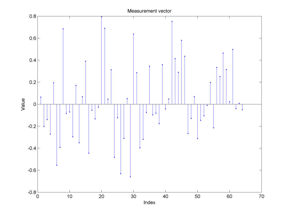
Making random measurements from sparse high dimensional vector:
y0 = Phi * x;
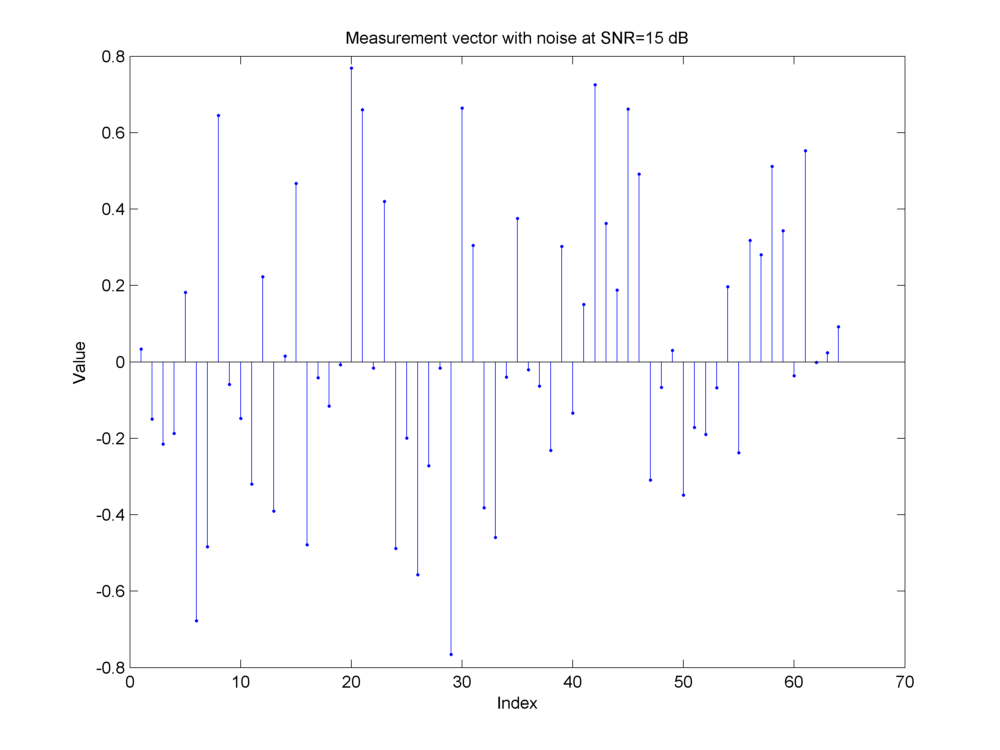
Adding some measurement noise:
SNR = 15;
snr = db2pow(SNR);
noise = randn(M, 1);
% we treat each column as a separate data vector
signalNorm = norm(y0);
noiseNorm = norm(noise);
actualNormRatio = signalNorm / noiseNorm;
requiredNormRatio = sqrt(snr);
gain_factor = actualNormRatio  / requiredNormRatio;
noise = gain_factor .* noise;
Measurement vector with noise:
y = y0 + noise;
Sparse recovery using matching pursuit:
solver = spx.pursuit.single.MatchingPursuit(Phi, K);
result = solver.solve(y);
mp_solution = result.z;
Recovery error:
mp_diff = x - mp_solution;
mp_recovery_error = norm(mp_diff) / norm(x);
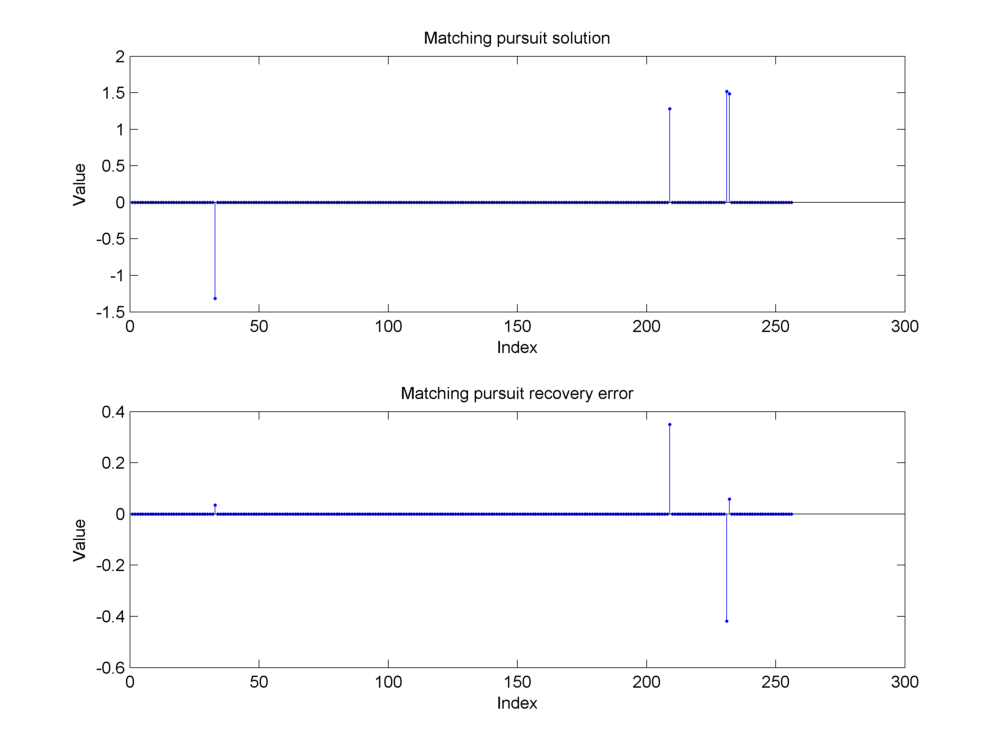
Matching pursuit recovery error: 0.1612.
Sparse recovery using orthogonal matching pursuit:
solver = spx.pursuit.single.OrthogonalMatchingPursuit(Phi, K);
result = solver.solve(y);
omp_solution = result.z;
omp_diff = x - omp_solution;
omp_recovery_error = norm(omp_diff) / norm(x);
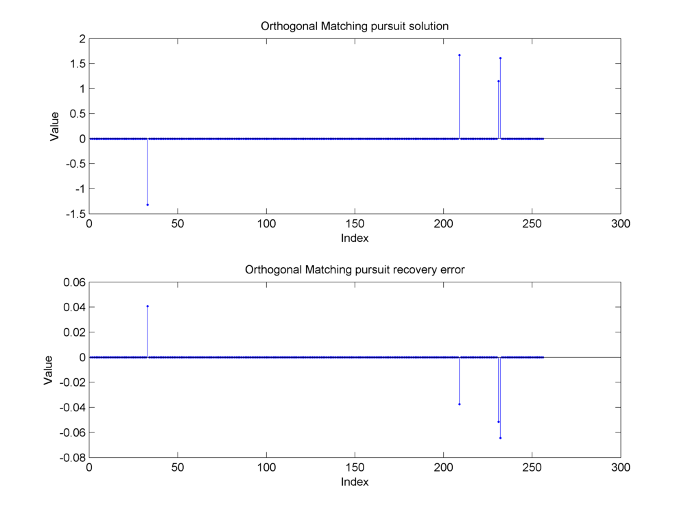
Orthogonal Matching pursuit recovery error: 0.0301.
Sparse recovery using l_1 minimization:
solver = spx.pursuit.single.BasisPursuit(Phi, y);
result = solver.solve_l1_noise();
l1_solution = result;
l1_diff = x - l1_solution;
l1_recovery_error = norm(l1_diff) / norm(x);
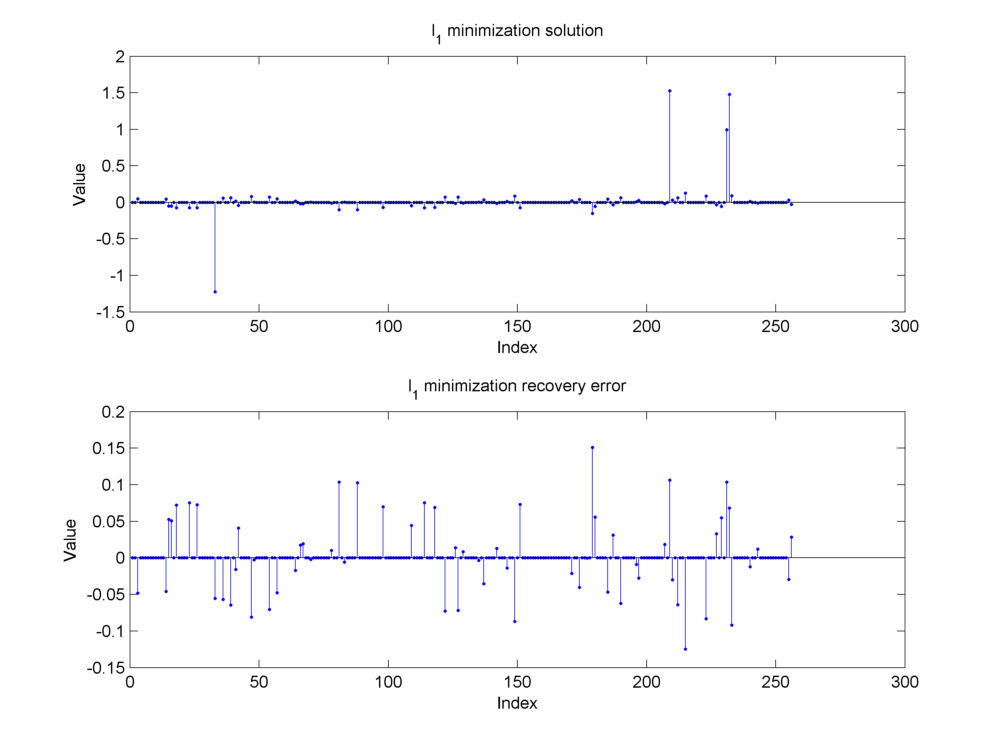
l_1 recovery error: 0.1764.