Matching Pursuit Algorithm¶

Matching Pursuit

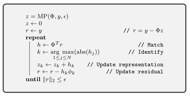
The matching pursuit algorithm is a very simple iterative approach to solve the sparse recovery problem. We are given the signal \(y\) and the dictionary \(\Phi\) and we are to recover the sparse representation \(x\) satisfying \(y = \Phi x\).

In each iteration of matching pursuit:

A current estimate of the representation vector \(x\) is maintained in the variable \(z\).
Current residual \(r = y - \Phi z\) is maintained.
The inner product of the residual with all the atoms in \(\Phi\) is computed.
We look for the atom which has the largest inner product in magnitude.
Contribution from this atom is added to the representation.
Residual is reduced accordingly.

Note that it is guaranteed that the norm of residual decreases monotonically in each iteration till it converges.

The algorithm can be motivated as follows.

Let \(\Lambda\) be the support of the representation vector \(x\). Then

\[y = \sum_{j \in \Lambda} \phi_{j} x_{j}.\]

For some \(k \in \Lambda\)

\[\langle y, \phi_k \rangle = \sum_{j \in \Lambda} \langle \phi_{j} , \phi_k \rangle x_{j}.\]

If the atoms formed an orthonormal set, this would have reduced to \(x_{k} = \langle y, \phi_k \rangle\) and picking the largest inner product would give us the largest non-zero entry in \(x\).

In fact, if \(\Phi\) was an orthonormal basis, then matching pursuit recovers the representation of \(y\) in exactly \(K\) iterations where \(K = |\Lambda|\) by successively picking up nonzero coefficients in \(x\) in the order of descending magnitude. We hope that the algorithm is useful even when the atoms in \(\Phi_{\Lambda}\) are not orthogonal.

Now, let us look at the iterative structure. Assume that the current estimate \(z\) satisfies \(\supp(z) \subseteq \Lambda\). Then \(\Phi z \in \Range(\Phi_{\Lambda})\). Since \(y \in \Range(\Phi_{\Lambda})\), hence the residual \(r \in \Range(\Phi_{\Lambda})\) also holds.

Finally, if the atoms in \(\Phi\) are nearly orthogonal to each other, then the largest inner product of \(r\) will be for one of the atoms in \(\Lambda\). This atom is indexed by the variable \(k\). Then \(h_k\) is the projection of the residual \(r\) on the atom \(\phi_k\).

We add this projection coefficient to \(z_k\) and remove the projection from the residual. The support of \(z\) continues to be within \(\Lambda\).

Since the atoms are not orthogonal, matching pursuit typically takes much larger number of iterations than the sparsity level \(K\). However, under suitable conditions, it does converge to the correct solution.

Hands-on with Matching Pursuit¶

Matching pursuit on a 2-sparse vector¶

In this example, we will reconstruct a 2-sparse representation vector \(x\) from a signal \(y = \Phi x\). We will develop the basic implementation of matching pursuit along-with.

From this example, we know of a way to construct a dictionary with high spark:

rng default;
N = 20;
M = 10;
K = 2;
PhiA = hadamard(N);
rows = randperm(N, M);
PhiB = PhiA(rows, :);

Let’s print its contents:

>> PhiB

PhiB =

-1 -1 -1 -1  1 -1  1 -1  1  1  1  1 -1 -1  1 -1 -1  1  1
-1 -1  1 -1 -1  1  1 -1 -1 -1 -1  1 -1  1 -1  1  1  1  1
-1 -1 -1  1 -1  1 -1  1  1  1  1 -1 -1  1 -1 -1  1  1 -1
1  1 -1 -1  1 -1 -1  1  1 -1 -1 -1 -1  1 -1  1 -1  1  1
1 -1  1  1  1  1 -1 -1  1 -1 -1  1  1 -1 -1 -1 -1  1 -1
-1  1  1  1  1 -1 -1  1 -1 -1  1  1 -1 -1 -1 -1  1 -1  1
-1  1  1 -1 -1 -1 -1  1 -1  1 -1  1  1  1  1 -1 -1  1 -1
1  1 -1 -1 -1 -1  1 -1  1 -1  1  1  1  1 -1 -1  1 -1 -1
-1  1 -1 -1  1  1 -1 -1 -1 -1  1 -1  1 -1  1  1  1  1 -1
1 -1 -1  1  1 -1 -1 -1 -1  1 -1  1 -1  1  1  1  1 -1 -1

Let’s normalize its columns:

Phi = spx.norm.normalize_l2(PhiB);

Bi-Gaussian discusses ways to generate synthetic sparse vectors.

Let’s generate our 2-sparse representation vector:

rng(100);
gen = spx.data.synthetic.SparseSignalGenerator(N, K);
x =  gen.biGaussian();

Let’s print \(x\):

>> spx.io.print.sparse_signal(x);
(6,1.6150) (11,-1.2390)   N=20, K=2

This is a nice helper function to print sparse vectors. It prints a sequence of tuples where each tuple consists of the index of a non-zero value and corresponding value.

The support for this vector is:

>> spx.commons.sparse.support(x)'

ans =

     6    11

Let’s construct our 10-dimensional signal from it:

y = Phi * x;

Let’s print it:

>> spx.io.print.vector(y)
0.12 -0.12 -0.90 0.90 0.90 0.90 -0.90 -0.12 0.90 0.12

Our problem is now setup. Our job now is to recover \(x\) from \(\Phi\) and \(y\).

Initialize the estimated representation and current residual:

z = zeros(N, 1);
r = y;

We will run the matching pursuit iterations up to 100 times:

for i=1:100

Following code samples are part of each matching pursuit iteration. We start with computing the inner products of the current residual with each atom:

inner_products = Phi' * r;

Find the index of best matching atom \(k\)

[max_abs_inner_product, index]  = max(abs(inner_products));

Corresponding signed inner product \(h_k\):

max_inner_product = inner_products(index);

Update the representation:

z(index) = z(index) + max_inner_product;

Remove the projection of the atom from the residual:

r = r - max_inner_product * Phi(:, index);

Compute the norm of residual:

norm_residual = norm(r);

If the norm is less than a threshold, we break out of loop:

if norm_residual < 1e-4
    break;
end

It will be instructive to print current value of residual norm, selected atom index and estimated coefficients in the \(z\) variable in each iteration:

fprintf('[%d]: k: %d, h_k : %.4f, r_norm: %.4f, estimate: ', i, index, norm_residual, max_inner_product);

Here is the output of running this algorithm for this problem:

[1]: k: 6, h_k : 1.2140, r_norm: 1.8628, estimate: (6,1.8628)   N=20, K=1
[2]: k: 11, h_k : 0.2428, r_norm: -1.1894, estimate: (6,1.8628) (11,-1.1894)   N=20, K=2
[3]: k: 6, h_k : 0.0486, r_norm: -0.2379, estimate: (6,1.6249) (11,-1.1894)   N=20, K=2
[4]: k: 11, h_k : 0.0097, r_norm: -0.0476, estimate: (6,1.6249) (11,-1.2370)   N=20, K=2
[5]: k: 6, h_k : 0.0019, r_norm: -0.0095, estimate: (6,1.6154) (11,-1.2370)   N=20, K=2
[6]: k: 11, h_k : 0.0004, r_norm: -0.0019, estimate: (6,1.6154) (11,-1.2389)   N=20, K=2
[7]: k: 6, h_k : 0.0001, r_norm: -0.0004, estimate: (6,1.6150) (11,-1.2389)   N=20, K=2

It took us 7 iterations, but the residual norm reached close to 0. We can note that the non-zero values in \(z\) match closely with the corresponding values in \(x\). Matching pursuit has been successful. We can also notice that the reconstruction alternates between atom number 6 and 11 in each iteration. Also, the residual norm keeps on decreasing with each iteration.

The complete code can be downloaded here.

ExampleWhen matching pursuit fails::

Although the spark of the dictionary in previous example is \(8\), matching pursuit fails to recover signals which are 3-sparse.

Here is an example output of running matching pursuit on a 3-sparse vector for 20 iterations:

The representation: (6,-1.9014) (8,1.3481) (11,1.6150)   N=20, K=3
[1]: k: 6, h_k : 1.9189, r_norm: -2.7636, estimate: (6,-2.7636)   N=20, K=1
[2]: k: 11, h_k : 1.2654, r_norm: 1.4425, estimate: (6,-2.7636) (11,1.4425)   N=20, K=2
[3]: k: 8, h_k : 0.7712, r_norm: 1.0032, estimate: (6,-2.7636) (8,1.0032) (11,1.4425)   N=20, K=3
[4]: k: 6, h_k : 0.3449, r_norm: 0.6898, estimate: (6,-2.0738) (8,1.0032) (11,1.4425)   N=20, K=3
[5]: k: 8, h_k : 0.2069, r_norm: 0.2759, estimate: (6,-2.0738) (8,1.2791) (11,1.4425)   N=20, K=3
[6]: k: 11, h_k : 0.1542, r_norm: 0.1380, estimate: (6,-2.0738) (8,1.2791) (11,1.5805)   N=20, K=3
[7]: k: 6, h_k : 0.0690, r_norm: 0.1380, estimate: (6,-1.9359) (8,1.2791) (11,1.5805)   N=20, K=3
[8]: k: 8, h_k : 0.0414, r_norm: 0.0552, estimate: (6,-1.9359) (8,1.3343) (11,1.5805)   N=20, K=3
[9]: k: 16, h_k : 0.0308, r_norm: 0.0276, estimate: (6,-1.9359) (8,1.3343) (11,1.5805) (16,0.0276)   N=20, K=4
[10]: k: 14, h_k : 0.0241, r_norm: -0.0193, estimate: (6,-1.9359) (8,1.3343) (11,1.5805) (14,-0.0193) (16,0.0276)
  N=20, K=5
[11]: k: 10, h_k : 0.0197, r_norm: 0.0138, estimate: (6,-1.9359) (8,1.3343) (10,0.0138) (11,1.5805) (14,-0.0193)
(16,0.0276)   N=20, K=6
[12]: k: 6, h_k : 0.0151, r_norm: 0.0127, estimate: (6,-1.9232) (8,1.3343) (10,0.0138) (11,1.5805) (14,-0.0193)
(16,0.0276)   N=20, K=6
[13]: k: 11, h_k : 0.0115, r_norm: 0.0097, estimate: (6,-1.9232) (8,1.3343) (10,0.0138) (11,1.5902) (14,-0.0193)
(16,0.0276)   N=20, K=6
[14]: k: 15, h_k : 0.0095, r_norm: -0.0065, estimate: (6,-1.9232) (8,1.3343) (10,0.0138) (11,1.5902) (14,-0.0193)
(15,-0.0065) (16,0.0276)   N=20, K=7
[15]: k: 13, h_k : 0.0078, r_norm: 0.0055, estimate: (6,-1.9232) (8,1.3343) (10,0.0138) (11,1.5902) (13,0.0055)
(14,-0.0193) (15,-0.0065) (16,0.0276)   N=20, K=8
[16]: k: 1, h_k : 0.0056, r_norm: -0.0054, estimate: (1,-0.0054) (6,-1.9232) (8,1.3343) (10,0.0138) (11,1.5902)
(13,0.0055) (14,-0.0193) (15,-0.0065) (16,0.0276)   N=20, K=9
[17]: k: 20, h_k : 0.0044, r_norm: -0.0035, estimate: (1,-0.0054) (6,-1.9232) (8,1.3343) (10,0.0138) (11,1.5902)
(13,0.0055) (14,-0.0193) (15,-0.0065) (16,0.0276) (20,-0.0035)
  N=20, K=10
[18]: k: 2, h_k : 0.0034, r_norm: 0.0028, estimate: (1,-0.0054) (2,0.0028) (6,-1.9232) (8,1.3343) (10,0.0138)
(11,1.5902) (13,0.0055) (14,-0.0193) (15,-0.0065) (16,0.0276)
(20,-0.0035)   N=20, K=11
[19]: k: 4, h_k : 0.0025, r_norm: 0.0023, estimate: (1,-0.0054) (2,0.0028) (4,0.0023) (6,-1.9232) (8,1.3343)
(10,0.0138) (11,1.5902) (13,0.0055) (14,-0.0193) (15,-0.0065)
(16,0.0276) (20,-0.0035)   N=20, K=12
[20]: k: 17, h_k : 0.0021, r_norm: -0.0014, estimate: (1,-0.0054) (2,0.0028) (4,0.0023) (6,-1.9232) (8,1.3343)
(10,0.0138) (11,1.5902) (13,0.0055) (14,-0.0193) (15,-0.0065)
(16,0.0276) (17,-0.0014) (20,-0.0035)   N=20, K=13

The sparse vector is supported on atoms 6, 8 and 11. If we order the atoms in terms of the magnitude of their coefficients, the order is 6,11 and 8.

Atom 6 is discovered in first iteration.
Atom 11 is discovered in second iteration.
Atom 8 is discovered in the third iteration.
The coefficients for atom 6, 8 and 11 continue to be updated till 8 iterations.
In 9-th iteration, it discovers an incorrect atom 16.
In the following iterations, it keeps discovering more incorrect atoms 14, 10, 15, 13, 1, 20, etc.
The algorithm is side-tracked after 9-th iteration. The residual doesn’t belong to the range \(\Range(\Phi_{\Lambda})\) anymore.
After 20 iterations, as many as 13 atoms are involved in the representation.
Yet, most of the energy is concentrated in atoms 6, 8, 11 only. In that sense, MP hasn’t failed completely.
A simple thresholding can remove the spurious contributions from incorrect atoms.