Working with Daubechies Wavelets

The short name for this family of wavelets is db.

Information about the wavelet family:

>> waveinfo('db')
 Information on Daubechies wavelets.

    Daubechies Wavelets

    General characteristics: Compactly supported
    wavelets with extremal phase and highest
    number of vanishing moments for a given
    support width. Associated scaling filters are
    minimum-phase filters.

    Family                  Daubechies
    Short name              db
    Order N                 N a positive integer from 1 to 45.
    Examples                db1 or haar, db4, db15

    Orthogonal              yes
    Biorthogonal            yes
    Compact support         yes
    DWT                     possible
    CWT                     possible

    Support width           2N-1
    Filters length          2N
    Regularity              about 0.2 N for large N
    Symmetry                far from
    Number of vanishing
    moments for psi         N

    Reference: I. Daubechies,
    Ten lectures on wavelets,
    CBMS, SIAM, 61, 1994, 194-202.

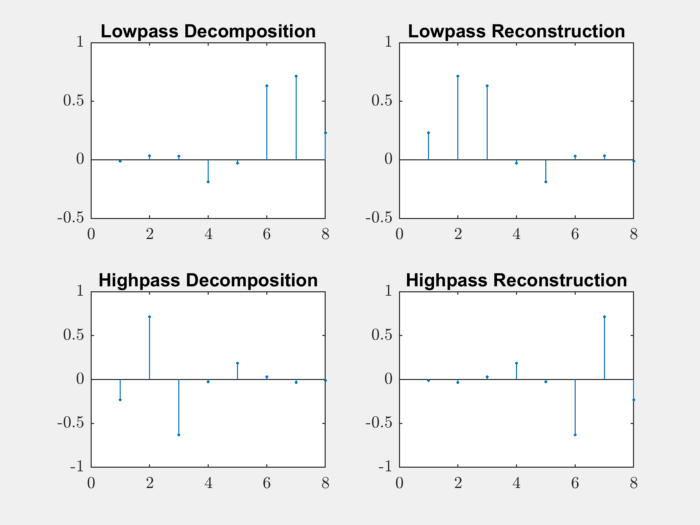
Decomposition and Reconstruction filters

Let’s construct the filters for ‘db4’ wavelet:

>> [LoD,HiD,LoR,HiR] = wfilters('db4');

Let’s plot the filters:

subplot(221);
stem(LoD, '.'); title('Lowpass Decomposition');
subplot(222);
stem(LoR,'.'); title('Lowpass Reconstruction');
subplot(223);
stem(HiD,'.'); title('Highpass Decomposition');
subplot(224);
stem(HiR,'.'); title('Highpass Reconstruction');

Single Level Decomposition and Reconstruction

The dwt and idwt functions can be used for single level decomposition and reconstruction.

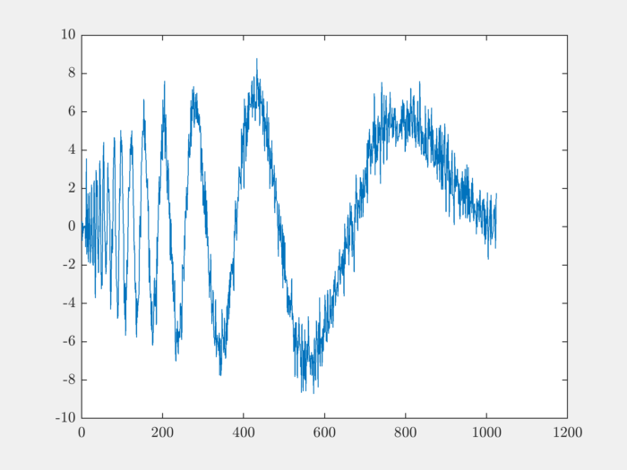
Let’s load a signal on which we will perform the decomposition:

load noisdopp;
plot(noisdopp);

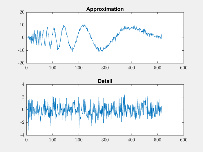
Let’s perform 1-level decomposition:

[approximation, detail] = dwt(noisdopp,LoD,HiD);

Let’s plot the decomposed approximation and detail components:

subplot(211);
plot(approximation); title('Approximation');
subplot(212);
plot(detail); title('Detail');

Reconstruct the original signal using idwt:

reconstructed = idwt(approximation, detail,LoR,HiR);

Let’s measure the reconstruction error:

>> max_abs_diff = max(abs(noisdopp-reconstructed))

max_abs_diff =

   6.3300e-12

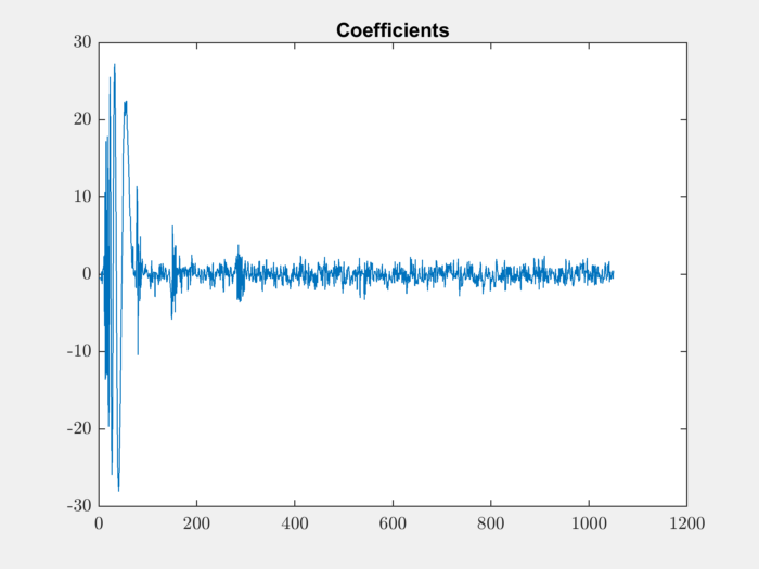
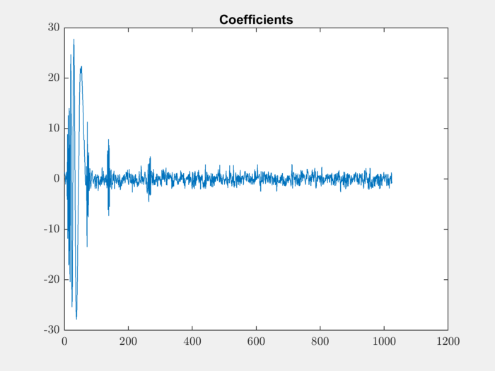
Multi-level Wavelet Decomposition

We can use the wavedec function for multi-level wavelet decomposition:

[coefficients, levels] = wavedec(s,3,'db1');

Let’s plot the decomposition coefficients:

plot(coefficients); title('Coefficients');

Reconstruction from multi-level decomposition:

reconstructed = waverec(coefficients, levels, LoR, HiR);

Let’s verify the reconstruction error:

max_abs_diff = max(abs(noisdopp-reconstructed))
max_abs_diff =

   2.0627e-11

It is possible to look at the approximation coefficients at all levels:

for level=0:4
    level_app_coeffs = appcoef(coefficients, levels, LoR, HiR, level);
    subplot(511+level);
    plot(level_app_coeffs);
    title(sprintf('Approximation coefficients @ level-%d', level));
end

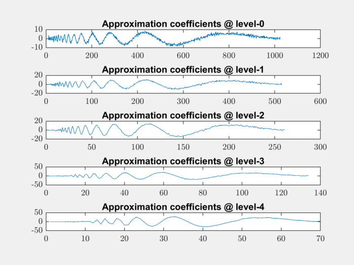
The level-0 coefficients are nothing but the original signal. The higher level approximation coefficients are increasingly smoother.

It is important to know how many levels of decomposition are possible. wmaxlev can be used for finding it out:

>> wmaxlev(numel(noisdopp),'db4')

ans =

     7

The normal wavelet decomposition creates more coefficients than there are in the original signal.

Let’s see how the number of coefficients increase with the level of decomposition:

>> for i=1:7
    [coefficients, levels] = wavedec(noisdopp,i, LoD,HiD);
    fprintf('%d ', numel(coefficients));
end

1030 1037 1044 1050 1056 1062 1068

For every level 6 or 7 extra coefficients are being introduced. This is because a normal convolution of length M signal with length N filter produces a signal of length M + N -1.

The behavior is controlled by the DWT MODE. It defines how the signals are extended to complete the convolution.

The default mode is:

>> dwtmode

*******************************************************
**  DWT Extension Mode: Symmetrization (half-point)  **
*******************************************************

Decomposition with Periodic Extension

If we want to have a non-redundant wavelet decomposition, we can use the periodic extension DWT mode.

Changing the mode:

old_dwt_mode = dwtmode('status','nodisp');
dwtmode('per');

*****************************************
**  DWT Extension Mode: Periodization  **
*****************************************

Performing level 4 decomposition:

[coefficients, levels] = wavedec(noisdopp,4, LoD,HiD);

Verify that the coefficients array is of same length as signal:

>> numel(coefficients)

ans =

        1024

Verify that number of elements at different levels is changing by a factor of 2 always:

>> levels

levels =

          64 64 128 256 512 1024

Plot the coefficients:

plot(coefficients); title('Coefficients');

Reconstruct the signal:

reconstructed = waverec(coefficients, levels, LoR, HiR);

Verify that the reconstruction is fine:

max_abs_diff = max(abs(noisdopp-reconstructed))

max_abs_diff =

   2.0357e-11

Plot the approximation coefficients at all levels:

for level=0:4
    level_app_coeffs = appcoef(coefficients, levels, LoR, HiR, level);
    subplot(511+level);
    plot(level_app_coeffs);
    fprintf('%d ', numel(level_app_coeffs));
    title(sprintf('Approximation coefficients @ level-%d', level));
end

1024 512 256 128 64

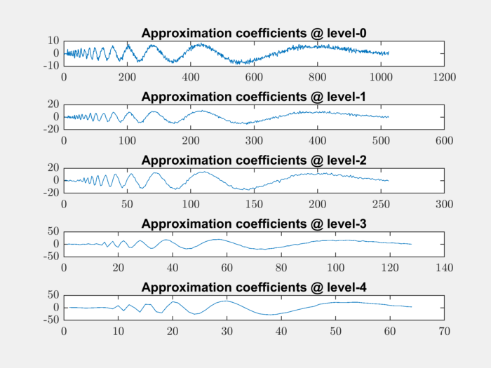
The number of approximation coefficients is decreasing exactly by a factor of 2 in each level.

Restoring the old DWT mode:

% restore the old DWT mode
dwtmode(old_dwt_mode);

Synthesis and Analysis Orthonormal Bases

Daubechies wavelets are orthogonal. For the specific case where the DWT is decomposing a signal \(x \in \RR^N\) to a representation \(\alpha \in \RR^N\) (in the periodic extension case), the transformation can be represented by an equation

\[x = \Psi \alpha\]

where \(\Psi\) is an Orthonormal basis (ONB) for \(\RR^N\) synthesizing the signal \(x\) from the representation \(\alpha\).

The decomposition process is represented by

\[\alpha = \Psi^T x.\]

We can easily construct the matrix \(\Psi^T\). Each column of \(\Psi^T\) can be obtained by computing \(\Psi^T e_i\) where \(e_i\) is the standard unit vector in i-th direction for \(\RR^N\).

We will construct the decomposition matrix for the ‘db4’ wavelet and level 4 decomposition. The size of the signal would be \(N=1024\):

[LoD,HiD,LoR,HiR] = wfilters('db4');

N = 1024;
L = 4;

Let’s make sure that we are using per mode:

old_dwt_mode = dwtmode('status','nodisp');
dwtmode('per');

Let’s construct \(\Psi^T\):

PsiT = zeros(N, N);
for i=1:N
    unit_vec = zeros(N, 1);
    unit_vec(i) = 1;
    [coefficients, levels] = wavedec(unit_vec, L, LoD,HiD);
    PsiT(:, i) = coefficients;
end

Let’s verify that the rows of \(\Psi^T\) are unit norm:

>> norms = spx.norm.norms_l2_rw(PsiT);
fprintf('norms: min: %.4f, max: %.4f\n', min(norms), max(norms));

norms: min: 1.0000, max: 1.0000

Let’s get the corresponding synthesis matrix \(\Psi\)

Psi = PsiT';

Let’s verify that it is indeed an orthonormal basis:

>> max(max(abs(Psi * Psi' - eye(N))))

ans =

   1.8573e-12

We should also verify that the matrix \(\Psi\) behaves same as the application of wavedec and waverec functions.

Let’s load our sample signal:

load noisdopp;
%  make it a column vector
noisdopp = noisdopp';

Let’s construct its representation by wavedec:

[a1, levels] = wavedec(noisdopp, L, LoD, HiD);

Let’s construct its representation by \(\Psi^T\):

a2 = PsiT * noisdopp;

Let’s compare if they match:

>> fprintf('Decomposition diff: %e\n', max(a1 - a2));
Decomposition diff: 2.486900e-14

They indeed match. Now, let’s reconstruct the signal through both ways. First using waverec:

x1  = waverec(a1, levels, LoR, HiR);

Now using \(\Psi\)

x2 = Psi * a2;

Compare them:

fprintf('Synthesis diff: %e\n', max(x1 - x2));
Synthesis diff: 1.065814e-14

It’s working great.

Finally, don’t forget to restore the older DWT mode:

dwtmode(old_dwt_mode);

It is instructive to visualize the basis \(\Psi\):

colormap('gray');
imagesc(Psi);
colorbar;

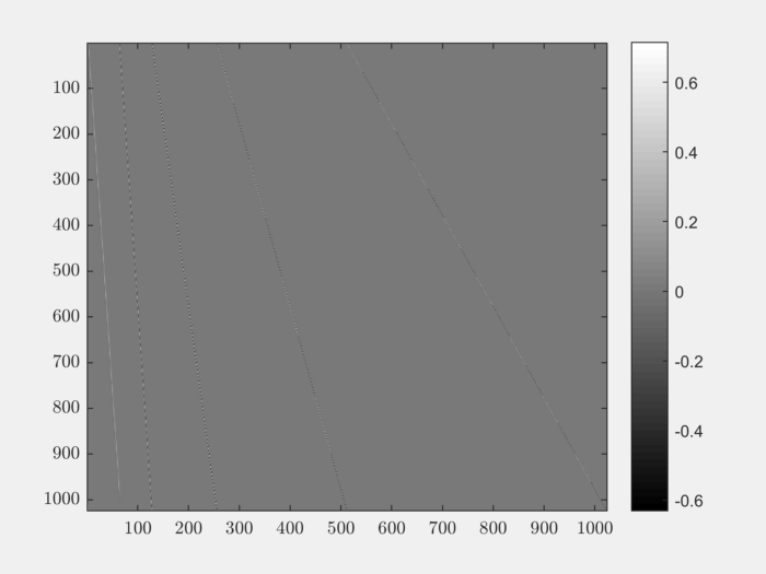
The matrix is sparse. In fact only 3% of its entries are non-zero:

>> nnz(Psi) / (N*N)

ans =

    0.0283

This is expected since wavelets have a very small support.

MATLAB provides a function for constructing a dictionary from one or more orthonormal or biorthogonal bases. Let’s try to construct a our ONB matrix using this function:

PsiMP = wmpdictionary(N, 'lstcpt', {{'db4', 4}});

Let’s verify that the two approaches are giving us same result:

>> max(max(abs(PsiMP - Psi)))

ans =

   7.9581e-13

A quick note, the wmpdictionary function returns a sparse matrix.

Complete example code can be downloaded here.

Stationary Wavelet Transform

DWT is not translation invariant. In some applications, translation invariance is important. Stationary Wavelet Transform (SWT) overcomes this limitation. It removes all the upsamplers and downsamplers in DWT. It is a highly redundant transform.

In MATLAB, it is implemented using swt function.

swt doesn’t involve any downsampling. All details and approximations are of same length as the original signal.

swt is defined using periodic extension. The length of the approximation and detail coefficients computed at each level equals the length of the signal.

Let us construct a level 4 decomposition:

coefficients = swt(noisdopp, 4, LoD,HiD);

Let’s plot the approximation and detail coefficients:

for level=0:4
    subplot(511+level);
    plot(coefficients(level+1, :));
    title(sprintf('SWT Coefficients @level-%d', level));
end