Detecting Dual Tone Multi Frequency Signals

Highlights

Following Matlab functions are demonstrated in this article: envelope, pulsewidth, periodogram, findpeaks, meanfreq,

A Dual Tone Multi Frequency (DTMF) signal is the signal generated from the punch keys of an ordinary telephone.

Each signal consists of a low frequency and a high frequency.

The table below lists the frequencies used for various keys.

Key	Low frequency	High frequency
1	697	1209 Hz
2	697	1336
3	697	1477
4	770	1209
5	770	1336
6	770	1477
7	852	1209
8	852	1336
9	852	1477
0	941	1336
	941	1209
#	941	1477

Let’s create a DTMM signal for the sequence of symbols 4, 5, 0, 7:

[signal, fs] = spx.dsp.dtmf({'4', '5', '0', '7'});

The corresponding time stamps:

time = (0:(numel(signal) - 1)) / fs;

Let’s plot it:

plot(1e3*time, signal);
xlabel('Time (ms)');
ylabel('Amplitude');
grid on;

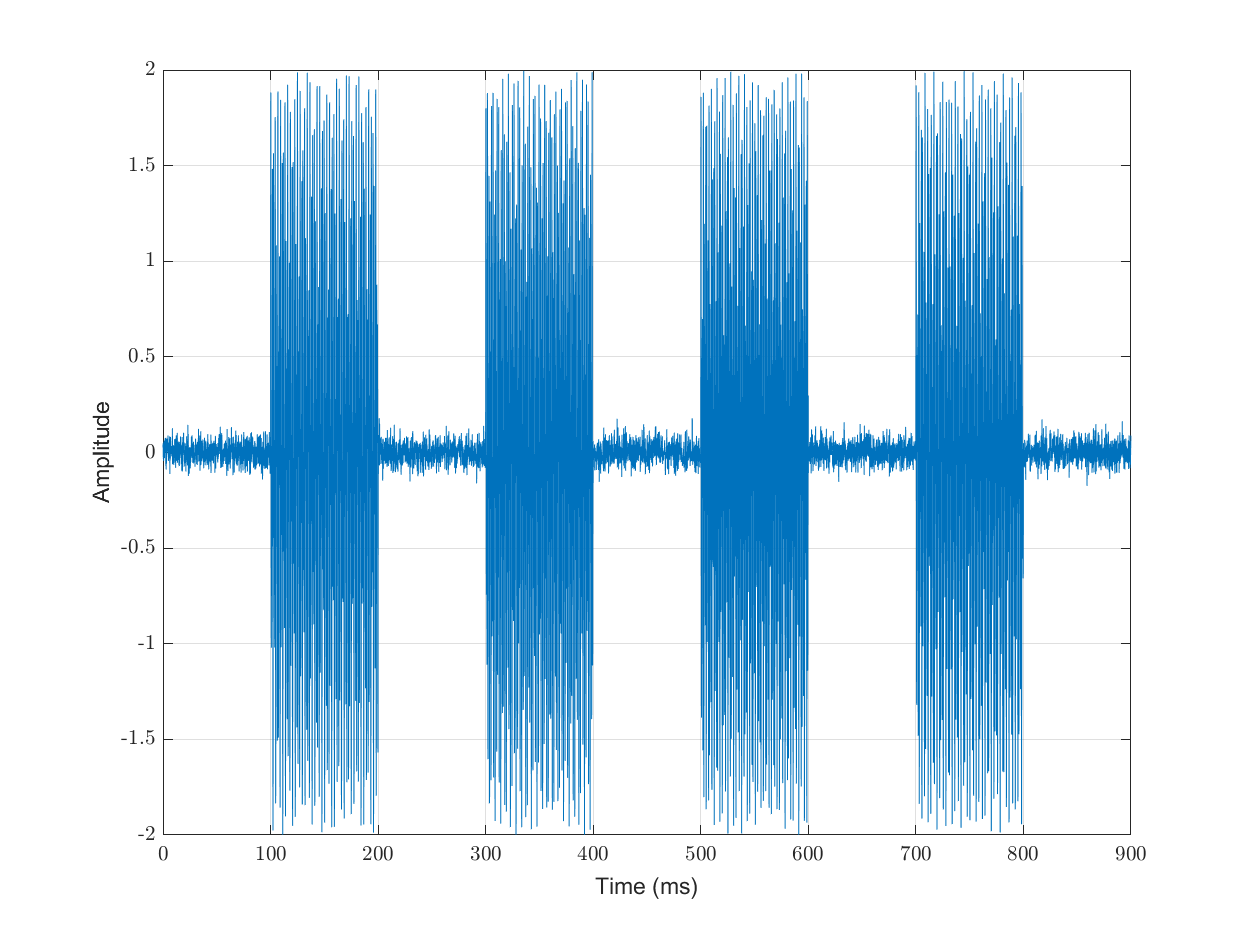
The pulses are 100 ms wide. The gap between pulses is also 100 ms wide and consists of Gaussian noise.

Our challenge would be to isolate the frequencies and identify the symbols transmitted.

Envelope

We can look at the shape of the pulses where the symbols were punched by looking at the RMS envelope of the signal:

envelope_signal = envelope(signal, 80,'rms');
plot(1e3*time, envelope_signal);

We are computing the RMS envelopes for window size of 80 samples.

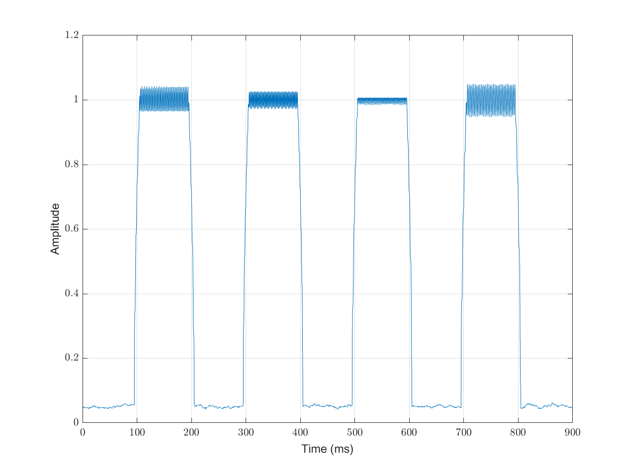
It is now easy to identify the pulses:

pulsewidth(envelope_signal,fs)
ans =

    0.1050
    0.1041
    0.1042
    0.1045

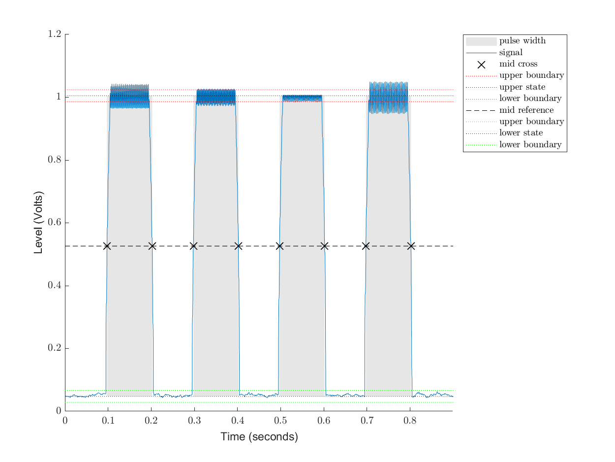
The recognized pulses are pretty close in size to the actual pulse size of 100 ms each.

Periodogram

A periodogram can help us identify the dominant frequencies present in the signal.

The frequencies involved in the sequence 4507 are 4 (770, 1209), 5(770, 1336), 0 (941, 1336), 7 (852, 1209).

We note that 770 Hz, 1209 Hz and 1336 Hz repeat twice, hence we expect them to have more contribution in the power spectrum. Other frequencies are 941 and 852 Hz.

Computing the periodogram is straight-forward:

[pxx,f]=periodogram(signal,[],[],fs);

Here is the display of power spectrum in deciBels.

We wish to isolate the peak frequencies from this plot:

[peak_values, peak_freqs] = findpeaks(pxx, f, 'SortStr','descend', 'MinPeakHeight', max(pxx) / 10);
peak_freqs = round(peak_freqs');

>> sort(peak_freqs)

ans =

Columns 1 through 9

766 771 774 853 941 1203 1205 1208 1210

Columns 10 through 14

1212 1215 1331 1335 1340

1. The frequencies 766, 771 and 774 are near 770 Hz.
2. 853 is near 852 Hz.
3. 941 matches 941 Hz.
4. 1203, 1205, 1208, 1210, 1212 and 1215 are near 1209 Hz.
5. 1331, 1335 and 1340 are near 1336 Hz.

Thus, the periodogram has been able to identify all the relevant frequencies in the signal and their power contribution appears to match well in their contribution in the constitution of the sequence 4502.

However, the periodogram is unable to localize the frequencies in time and hence is unable to tell us exactly which symbols were transmitted.

It is instructive to compute the mean frequencies in different bands:

>> round(meanfreq(pxx, f, 700 + [0, 100]))

ans =

   769

>> round(meanfreq(pxx, f, 800 + [0, 100]))

ans =

   851

>> round(meanfreq(pxx, f, 900 + [0, 100]))

ans =

   941

>> round(meanfreq(pxx, f, 1200 + [0, 100]))

ans =

        1211

>> round(meanfreq(pxx, f, 1300 + [0, 100]))

ans =

        1336

The mean frequencies in these bands are mostly spot-on or very close to actual frequencies sent in the DTMF signal.

Spectrogram

While, we have been able to identify the frequencies present in the signal, we haven’t been able to localize them in time. Thus, we are unable to identify exactly which symbols were sent.

The spectrogram provides us the time-frequency representation of the signal:

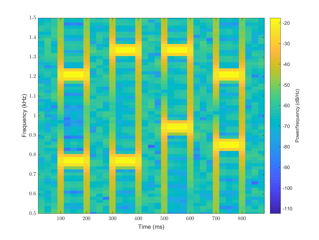
spectrogram(signal, [], [], [], fs, 'yaxis');
% restrict the y-axis between 500Hz to 1500 Hz.
ylim([0.5 1.5]);

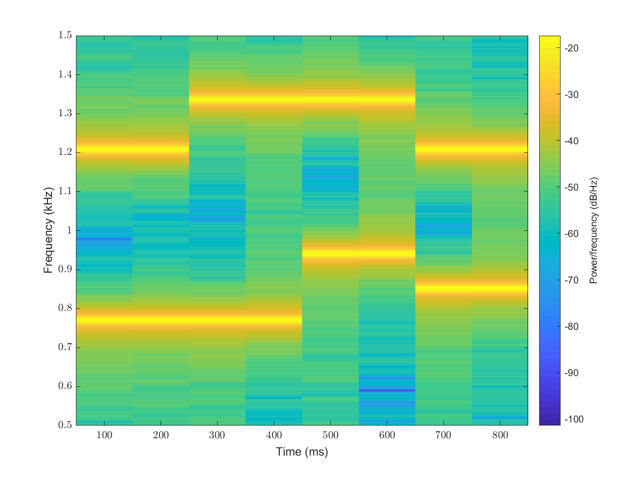
In this plot, it is clearly visible that at any point of time, two frequencies are active. There are four different symbols which seem to have been sent.

1. In the first symbol, the frequencies active seem to be around 770Hz and 1200 Hz which maps to the symbol 4.
2. In the second symbol, the frequencies active seem to be around 770Hz and 1330 Hz which maps to the symbol 5.
3. Similarly, we can see that the symbols 0 and 7 are easily visible in the spectrogram.

This spectrogram is not able to localize the symbols accurately. We are unable to see the portions where no symbols are being sent and only noise is present.

By default the spectrogram has following parameters:

• Signal is divided into segments which are around 22% of the length of the signal.
• The segments overlap each other by 50%.
• No windowing is done for computing the FFT of each segment.

We should increase the time resolution of the spectrogram.

Let’s have a window length of 50 ms:

window_length = floor(fs * 50 / 1000);

Let’s continue to have overlap of 50%:

overlap_length = floor(window_length / 2);

The FFT length depends on the window length:

n_fft = 2^nextpow2(window_length);

We will compute the spectrogram with Hamming window:

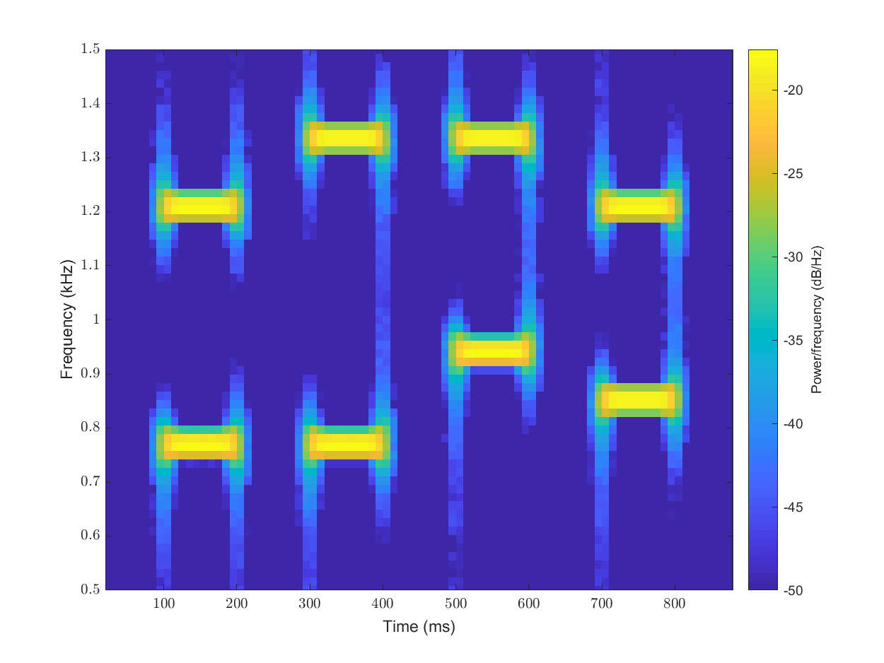
spectrogram(signal,hamming(window_length),overlap_length,n_fft, fs, 'yaxis');
ylim([0.5 1.5]);

Let’s visualize the results:

In this spectrogram, it is easy to see how the pulses in the signal are clearly visible and their frequencies can be easily read off the diagram.

While, we have improved time localization of pulses, the frequency localization has suffered a bit. Since, our interest is only in knowing the mean frequencies, this loss of frequency localization is not that important in this case.

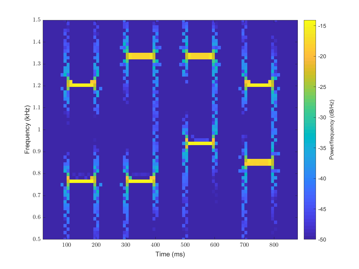
We can remove the frequencies which are contributing very small values to the spectrogram and enhance the prominent frequencies in the output. Also, we can increase the overlap between subsequent windows to introduce more spectrum lines and make the spectrogram look smoother:

overlap_length = floor(0.8 * window_length );
spectrogram(signal,hamming(window_length),overlap_length,n_fft, fs, 'yaxis', 'MinThreshold', -50);
ylim([0.5 1.5]);

By computing the center of energy for each spectral estimate in both time and frequency, we can do spectral reassignment. This gives us a much cleaner and crisper spectrogram.

Decoding the symbols

The complete process for decoding the DTMF sequence using the spectrogram has been implemented in the function spx.dsp.dtmf_decoder.

The function does the following:

• Compute the spectrogram
• Identify the times where spectral content has high energy
• Identify peak frequencies at these times
• Match these frequencies to the nearest low and high frequencies of DTMF sequences.
• Map the identified frequencies to actual symbols.
• Identify the start and duration of each symbol in terms of time.

You are welcome to look at the implementation.

We show the example use:

>> [symbols, starts, durations] = spx.dsp.dtmf_detector(signal, fs)

symbols =

  1×4 cell array

    {'4'}    {'5'}    {'0'}    {'7'}


starts =

    0.1000    0.3000    0.5000    0.7000


durations =

    0.1000    0.1000    0.1000    0.1000

Another example:

>> [signal, fs] = spx.dsp.dtmf({'2', '3', '4', '6', '*'});
>> [symbols, starts, durations] = spx.dsp.dtmf_detector(signal, fs)

symbols =

  1×5 cell array

    {'2'}    {'3'}    {'4'}    {'6'}    {'*'}


starts =

    0.1000    0.3000    0.5000    0.7000    0.9000


durations =

    0.1000    0.1000    0.1000    0.1000    0.1000