Hands-on spectral clustering
In this example, we will cluster 2D data which form three different rings in the plane.
Sample data is available in the data directory.
Let us load the data:
dataset_file = fullfile(spx.data_dir, 'clustering', ...
    'self_tuning_paper_clustering_data');
data = load(dataset_file);
datasets = data.XX;
raw_data = datasets{1};
num_clusters = data.group_num(1);
The raw data is organized in a matrix where each row represents one 2D point. Number of data points is the number of rows in the dataset. Let’s plot the data to get a better understanding:
X = raw_data(:, 1);
Y = raw_data(:, 2);
figure;
axis equal;
plot(X, Y, '.', 'MarkerSize',16);
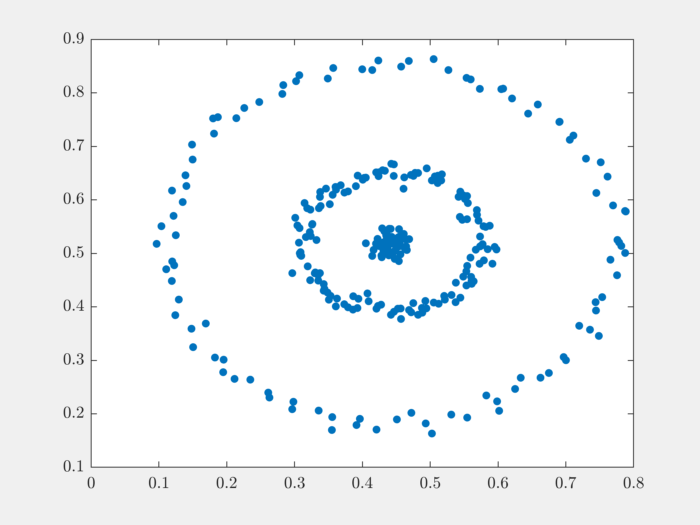
We can see that the data is organized in three different rings. This data set is unlikely to be clustered properly by K-means algorithm.
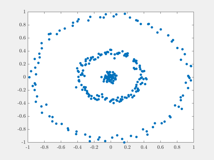
It is good practice to scale the data before clustering it:
raw_data = raw_data - repmat(mean(raw_data),size(raw_data,1),1);
raw_data = raw_data/max(max(abs(raw_data)));
X = raw_data(:, 1);
Y = raw_data(:, 2);
figure;
axis equal;
plot(X, Y, '.', 'MarkerSize',16);
The next step is to compute pairwise distances between the points in the dataset:
sqrt_dist_mat = spx.commons.distance.sqrd_l2_distances_rw(raw_data);
We convert the distances into a Gaussian similarity. To compute the similarity, we will need to provide the scale value:
scale = 0.04;
% Compute the similarity matrix
sim_mat = spx.cluster.similarity.gauss_sim_from_sqrd_dist_mat(sqrt_dist_mat, scale);
We are now ready to perform spectral clustering on the data.
Create the spectral clustering algorithm instance:
clusterer = spx.cluster.spectral.Clustering(sim_mat);
Inform it about the expected number of clusters:
clusterer.NumClusters = num_clusters;
There are two different spectral clustering algorithms available. We will use the random walk version:
cluster_labels = clusterer.cluster_random_walk();
We can summarize the results of clustering:
>> tabulate(cluster_labels)
  Value    Count   Percent
      1       99     33.11%
      2      139     46.49%
      3       61     20.40%
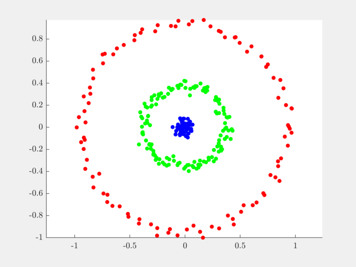
Let’s plot the data points in different colors depending on which cluster they belong to:
figure;
colors = [1,0,0;0,1,0;0,0,1;1,1,0;1,0,1;0,1,1;0,0,0];
hold on;
axis equal;
for c=1:num_clusters
    % Identify points in this cluster
    points = raw_data(cluster_labels == c, :);
    X = points(:, 1);
    Y = points(:, 2);
    plot(X, Y, '.','Color',colors(c,:), 'MarkerSize',16);
end
Complete example code can be downloaded
here.
Inside Unnormalized Spectral Clustering
In this section, we will start with a similarity matrix and go through the steps of unnormalized spectral clustering.
We will consider a simple case of of 8 data points which are known to be falling into two clusters.
We construct an undirected graph \(G\) where the nodes in same cluster are connected to each other and nodes in different clusters are not connected to each other.
In this simple example, we will assume that the graph is unweighted.
The adjacency matrix for the graph is \(W\):
>> W = [ones(4) zeros(4); zeros(4) ones(4)]
W =

     1     1     1     1     0     0     0     0
     1     1     1     1     0     0     0     0
     1     1     1     1     0     0     0     0
     1     1     1     1     0     0     0     0
     0     0     0     0     1     1     1     1
     0     0     0     0     1     1     1     1
     0     0     0     0     1     1     1     1
     0     0     0     0     1     1     1     1
We have arranged the adjacency matrix in a manner so that the clusters are easily visible.
Let’s just get the number of nodes:
>> [num_nodes, ~] = size(W);
Let’s also assign the true labels to these nodes which will be used for verification later:
>> true_labels = [1 1 1 1 2 2 2 2];
We construct the degree matrix \(D\) for the graph:
>> Degree = diag(sum(W))
Degree =

     4     0     0     0     0     0     0     0
     0     4     0     0     0     0     0     0
     0     0     4     0     0     0     0     0
     0     0     0     4     0     0     0     0
     0     0     0     0     4     0     0     0
     0     0     0     0     0     4     0     0
     0     0     0     0     0     0     4     0
     0     0     0     0     0     0     0     4
The unnormalized Laplacian is given by \(L = D - W\):
>> Laplacian = Degree - W
Laplacian =

     3    -1    -1    -1     0     0     0     0
    -1     3    -1    -1     0     0     0     0
    -1    -1     3    -1     0     0     0     0
    -1    -1    -1     3     0     0     0     0
     0     0     0     0     3    -1    -1    -1
     0     0     0     0    -1     3    -1    -1
     0     0     0     0    -1    -1     3    -1
     0     0     0     0    -1    -1    -1     3
We now compute the singular value decomposition of the Laplacian \(U \Sigma V^T = L\):
>> [~, S, V] = svd(Laplacian);
>> singular_values = diag(S);
>> fprintf('Singular values: \n');
>> spx.io.print.vector(singular_values);
Singular values:
4.00 4.00 4.00 4.00 4.00 4.00 0.00 0.00
We know that the number of connected components in an undirected graph is equal to the number of singular values of the Laplacian which are zero. On inspection, we can see that the there are indeed two such zeros.
For more general cases, the lower singular values may not indeed be zero. We need to find the knee of the singular value curve.
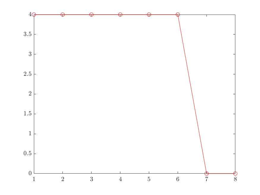
A simple way to find it to look at the changes between consecutive singular values and find the place where the change is largest:
>> sv_changes = diff( singular_values(1:end-1) );
>> spx.io.print.vector(sv_changes);
0.00 0.00 0.00 -0.00 0.00 -4.00
Note that it is known that the Laplacian always has one singular value which is 0. Thus, we need to look at the changes only in remaining singular values.
Locate the largest change:
>> [min_val , ind_min ] = min(sv_changes)
min_val =

   -4.0000


ind_min =

     6
The number of clusters is now easy to determine:
>> num_clusters = num_nodes - ind_min
num_clusters =

     2
We pickup the right singular vector corresponding to the last 2 smallest singular values:
>> Kernel = V(:,num_nodes-num_clusters+1:num_nodes);
Each row of this matrix corresponds to one data point. At this point, the standard k-means clustering can be invoked to cluster the points into clusters where the number of clusters was determined as above:
% Maximum iteration for KMeans Algorithm
>> max_iterations = 1000;
% Replication for KMeans Algorithm
>> replicates = 100;
>> labels = kmeans(Kernel, num_clusters, ...
    'start','sample', ...
    'maxiter',max_iterations,...
    'replicates',replicates, ...
    'EmptyAction','singleton'...
    );
Print the labels given by k-means:
>> spx.io.print.vector(labels, 0);
1 1 1 1 2 2 2 2
As expected, the algorithm has been able to group the points into two clusters. The labels are matching with the original true labels.
Complete example code can be downloaded
here.
sparse-plex includes a function
which implements the unnormalized
spectral clustering algorithm. We
can use it on the data above as follows:
>> result = spx.cluster.spectral.simple.unnormalized(W);
>> result.labels'

ans =

     1     1     1     1     2     2     2     2
Inside Normalized (Random Walk) Spectral Clustering
In this section, we will look at a spectral clustering method using normalized Laplacians. The primary difference is the way the graph Laplacian is computed \(L = I - D^{-1} W\).
We will use the third example from self tuning paper for demonstration here.
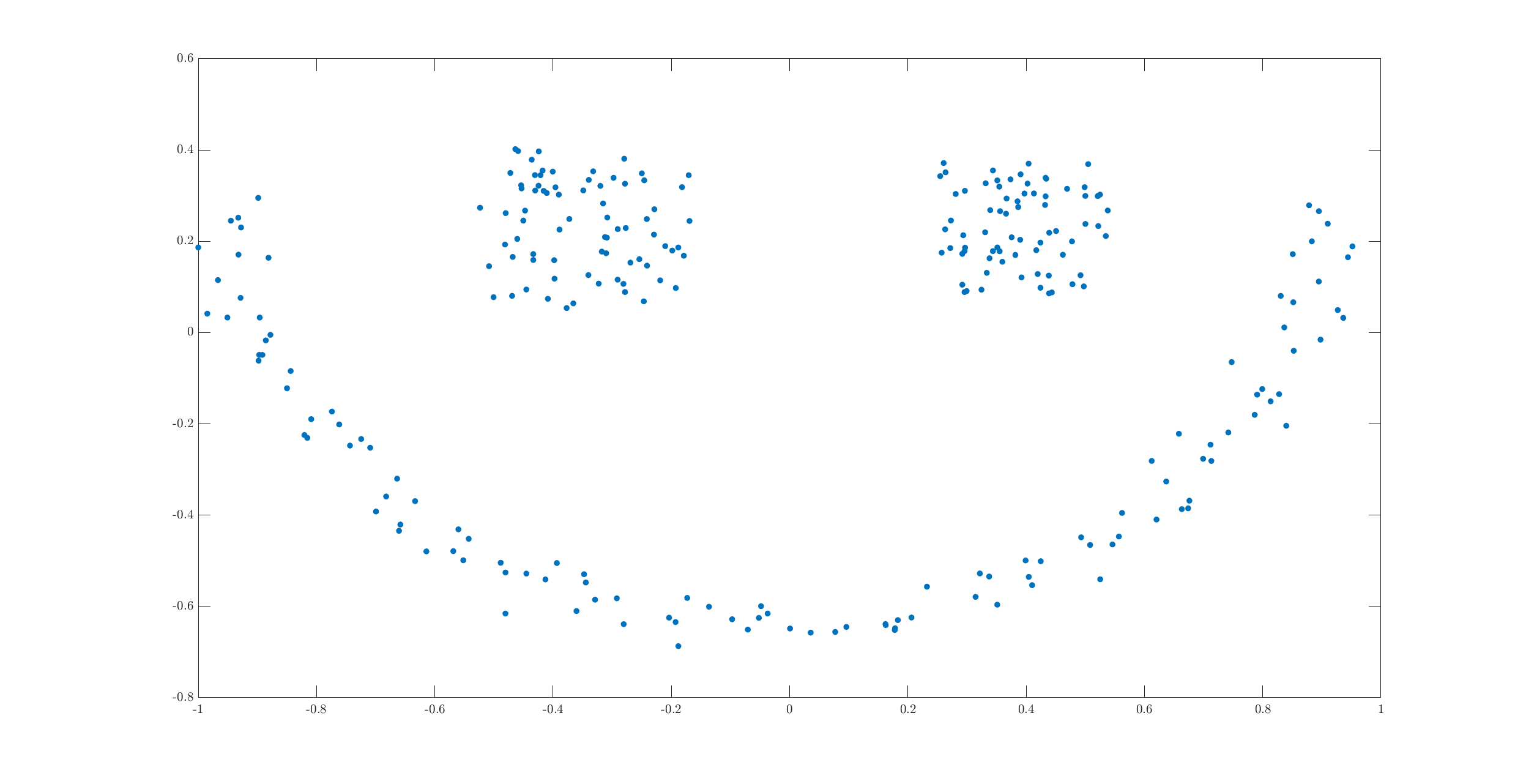
There are three clusters in the dataset. While two of the clusters have very clear convex shapes, the third one forms a half moon. It is this cluster which causes problems with a simple algorithm like k-means. The semi-moon is the first cluster, while the other two above it are cluster 2 and 3 (from left to right).
Loading the dataset:
dataset_file = fullfile(spx.data_dir, 'clustering', ...
    'self_tuning_paper_clustering_data');
data = load(dataset_file);
datasets = data.XX;
raw_data = datasets{3};
% Scale the raw_data
raw_data = raw_data - repmat(mean(raw_data),size(raw_data,1),1);
raw_data = raw_data/max(max(abs(raw_data)));
num_clusters = data.group_num(1);
X = raw_data(:, 1);
Y = raw_data(:, 2);
% plot it
axis equal;
plot(X, Y, '.', 'MarkerSize',16);
Let’s compute the pairwise (squared) \(\ell_2\) distances between the points:
sqrt_dist_mat = spx.commons.distance.sqrd_l2_distances_rw(raw_data);
imagesc(sqrt_dist_mat);
title('Distance Matrix');
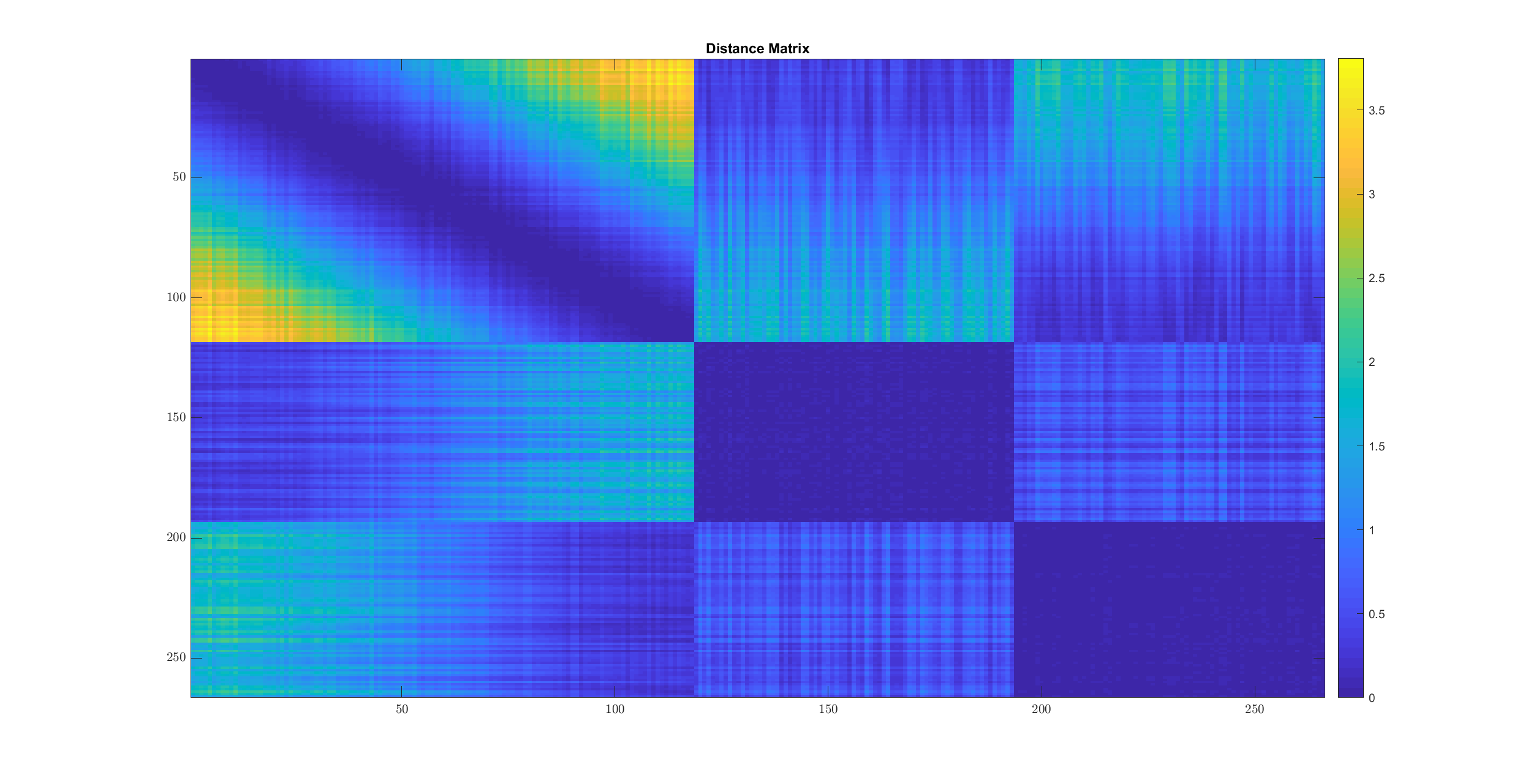
- In cluster 2 and 3, the distances are quite small between all pairs of points.
- In cluster 1, every point is near to some of the points. The points form kind of a chain structure. They keep getting farther and farther. This is visible from the gradual color change from blue to yellow in the off diagonal parts of the first (diagonal) sub-part in the image above.
We map the (squared) distances to similarity values between 0 to 1:
scale = 0.04;
W = spx.cluster.similarity.gauss_sim_from_sqrd_dist_mat(sqrt_dist_mat, scale);
imagesc(W);
title('Similarity Matrix');
The transformation involved here is
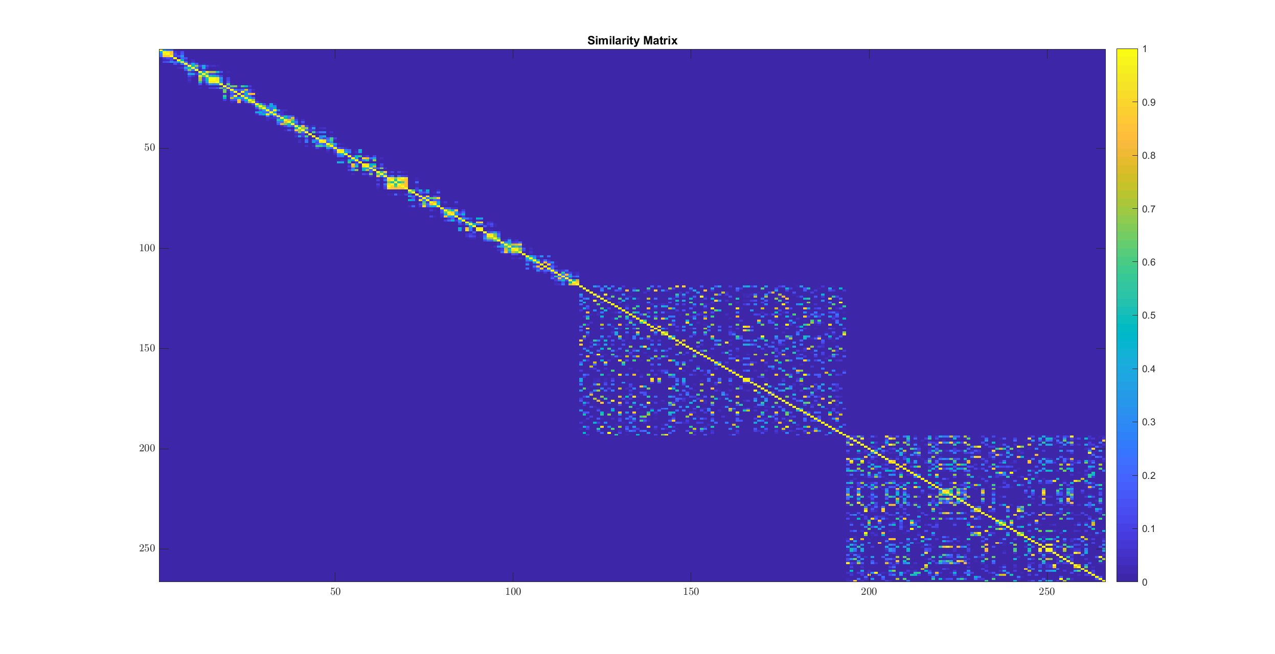
The chain structure of similarity in cluster 1 is clearly visible here. In cluster 2 and 3 points are fairly similar to each other.
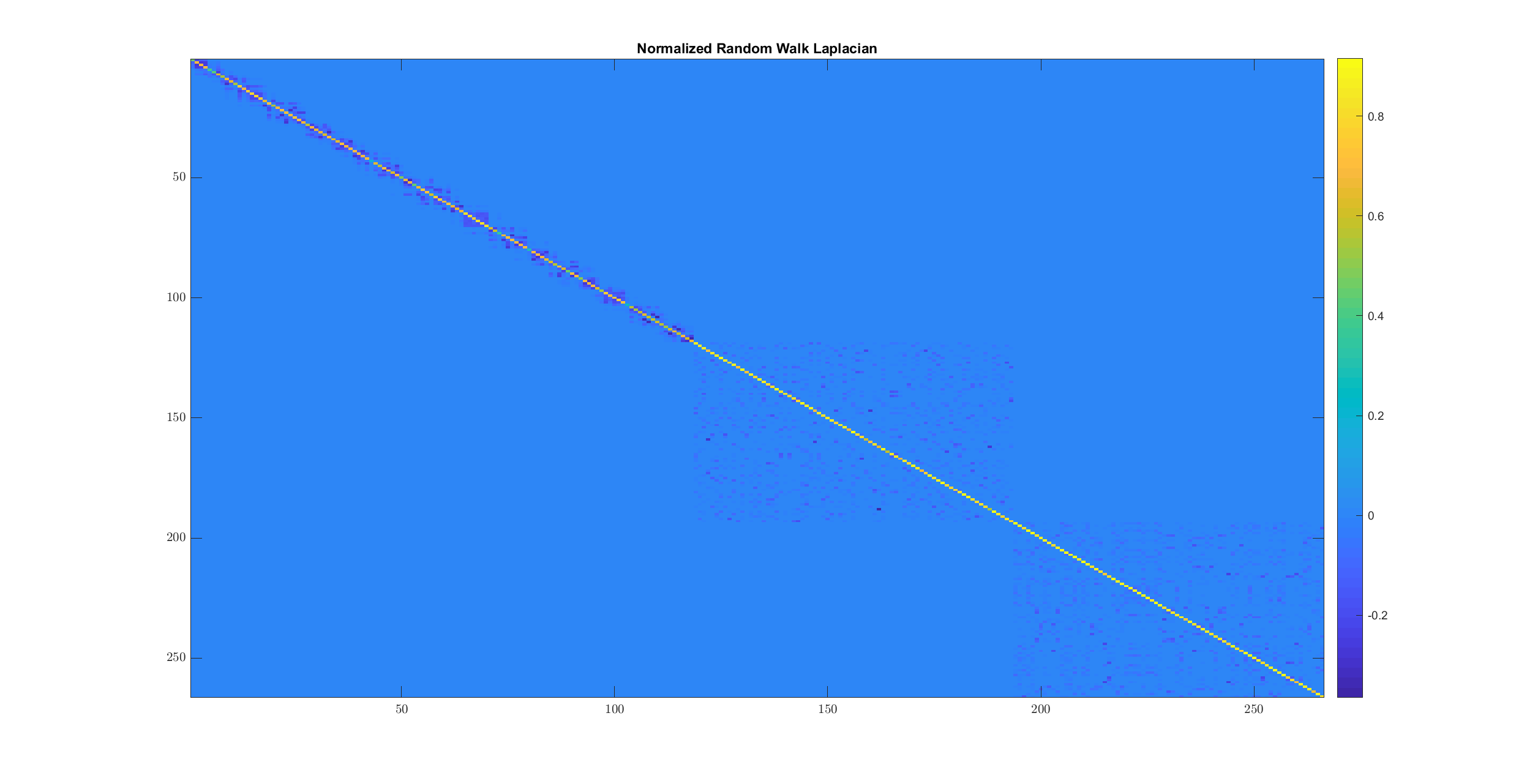
We now compute the graph Laplacian:
[num_nodes, ~] = size(W);
Degree = diag(sum(W));
DegreeInv = Degree^(-1);
Laplacian = speye(num_nodes) - DegreeInv * W;
imagesc(Laplacian);
title('Normalized Random Walk Laplacian');
Note how the Laplacian has been computed slightly differently.
Let’s look at the singular values:
[~, S, V] = svd(Laplacian);
singular_values = diag(S);
plot(singular_values, 'b.-');
grid on;
title('Singular values of the Laplacian');
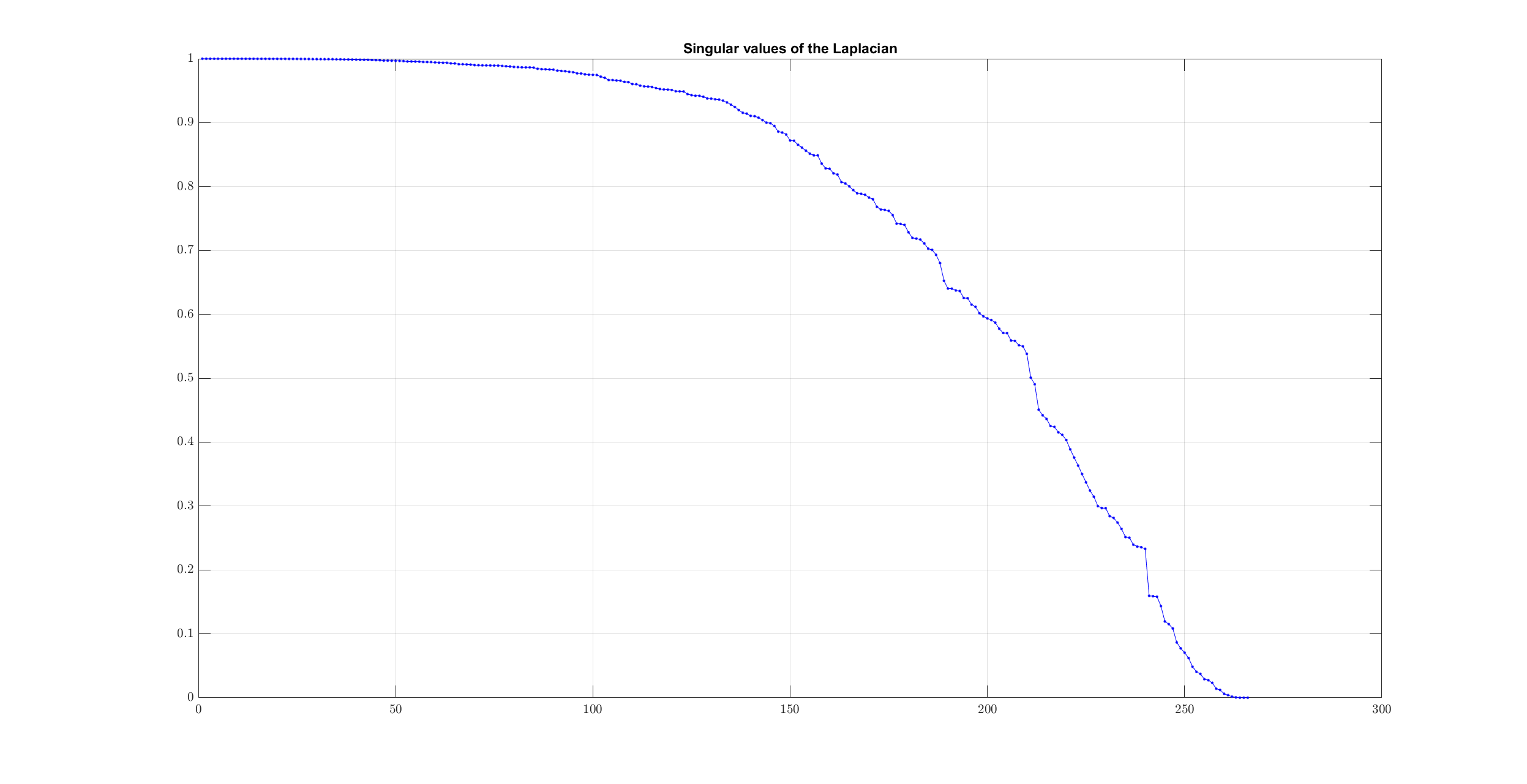
This time no clear knee is visible in the singular value plot. We can verify this by looking at the differences:
sv_changes = diff( singular_values(1:end-1) );
plot(sv_changes, 'b.-');
grid on;
title('Changes in singular values');
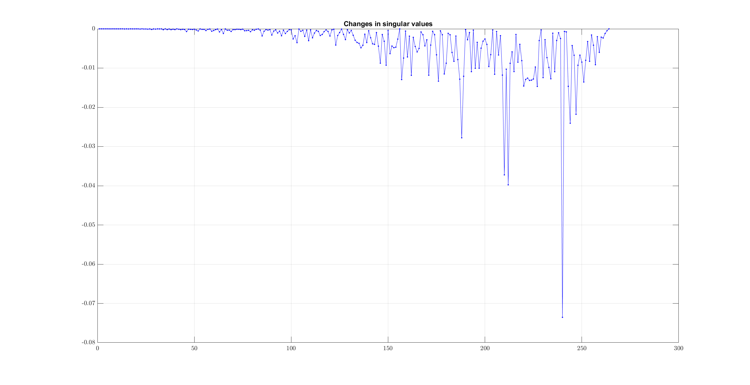
Finding the largest change in singular values will not give us the correct number of clusters:
>> [min_val , ind_min ] = min(sv_changes);
>> num_clusters = num_nodes - ind_min;
>> num_clusters

num_clusters =

    26
However, by data inspection, we can clearly see that there are only 3 clusters of interest.
In this case, since the data are well segregated, the number of singular values which is close to zero actually matches with the number of clusters:
>> num_clusters = sum(singular_values < 1e-6)
num_clusters =

     3
Let’s verify by printing 10 smallest singular values:
>> spx.io.print.vector(singular_values(end-10:end), 6)
0.027412 0.023242 0.014100 0.012101 0.006108 0.003988 0.001655 0.000471 0.000000 0.000000 0.000000
We will stick to this way of computing number of clusters here.
Let’s pick up the right singular vectors corresponding to the last 3 singular values:
% Choose the last num_clusters eigen vectors
Kernel = V(:,num_nodes-num_clusters+1:num_nodes);
Time to perform k-means clustering on the row vectors of this kernel:
% Maximum iteration for KMeans Algorithm
max_iterations = 1000;
% Replication for KMeans Algorithm
replicates = 100;
cluster_labels = kmeans(Kernel, num_clusters, ...
    'start','plus', ...
    'maxiter',max_iterations,...
    'replicates',replicates, ...
    'EmptyAction','singleton'...
    );
The labels are returned in the variable cluster_labels.
Let’s plot the original data by assigning different colors to points belonging to different labels:
hold on;
axis equal;
for c=1:num_clusters
    % Identify points in this cluster
    points = raw_data(cluster_labels == c, :);
    X = points(:, 1);
    Y = points(:, 2);
    plot(X, Y, '.', 'MarkerSize',16);
end
hold off;
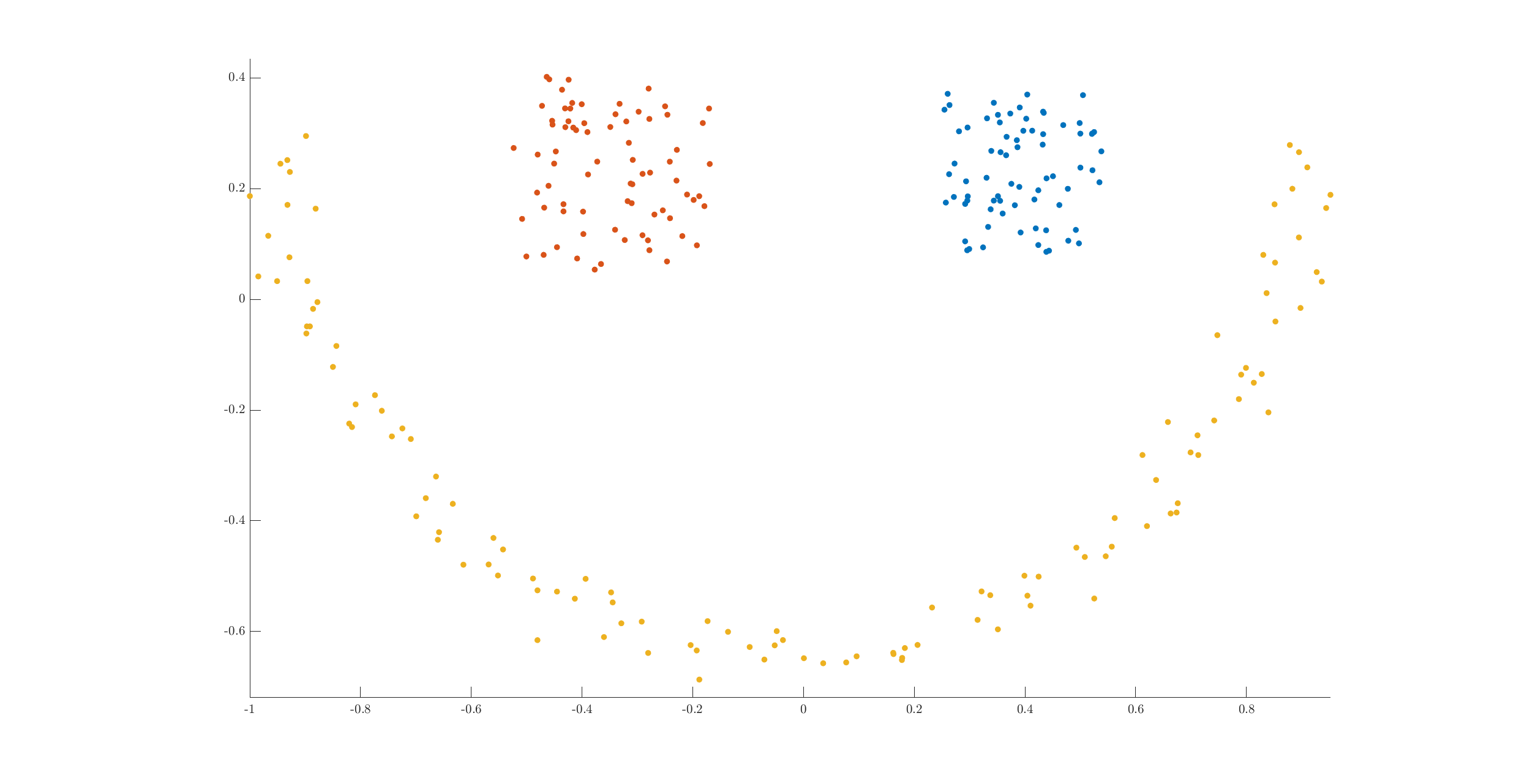
We can see that the clusters have been clearly identified.